【论文笔记】VI-Net: Boosting Category-level 6D Object Pose Estimation via Learning Decoupled Rotations on the Spherical Representations

VI-Net: Boosting Category-level 6D Object Pose Estimation via Learning Decoupled Rotations on the Spherical Representations

方法	类型	训练输入	推理输入	输出	pipeline
VI-Net	类别级	RGBD + 物体类别	RGBD + 物体类别	绝对\(\mathbf{R}, \mathbf{t}, \mathbf{s}\)

• 2025.04.01：类别级方法，使用一个网络估计旋转，另一个网络估计平移和缩放，24年CVPR SecondPose沿用了这个方法，对于旋转，该方法将旋转估计分为视角旋转和面内旋转，视作一个分类任务，分别估计，最后组合；对于平移和缩放，该方法使用PointNet++提取特征，直接估计平移和旋转

Abstract

1. Introduction

Figure 1. An illustration of the factorization of rotation \(\mathbf{R}\) into a viewpoint (out-of-plane) rotation \(\mathbf{R}_{vp}\) and an in-plane rotation \(\mathbf{R}_{ip}\) (around Z-axis). Notations are explained in Sec. 3.

Figure 2. An illustration of VI-Net for rotation estimation. We firstly construct a Spherical Feature Pyramid Network based on spatial spherical convolutions (SPA-SConv) to exact the high-level spherical feature map \(\mathcal{S}\). On top of \(\mathcal{S}\), a V-Branch is employed to search the canonical zenith direction on the sphere via binary classification for the generation of the viewpoint rotation \(\mathbf{R}_{vp}\), while another I-Branch is used to estimate the in-plane rotation \(\mathbf{R}_{ip}\) by transforming \(\mathcal{S}\) to view the object from the canonical zenith direction. Finally we have \(\mathbf{R} = \mathbf{R}_{vp}\mathbf{R}_{ip}\). Best view in the electronic version.

2. Related Work

3. Correlation on the Sphere and Rotation Decomposition

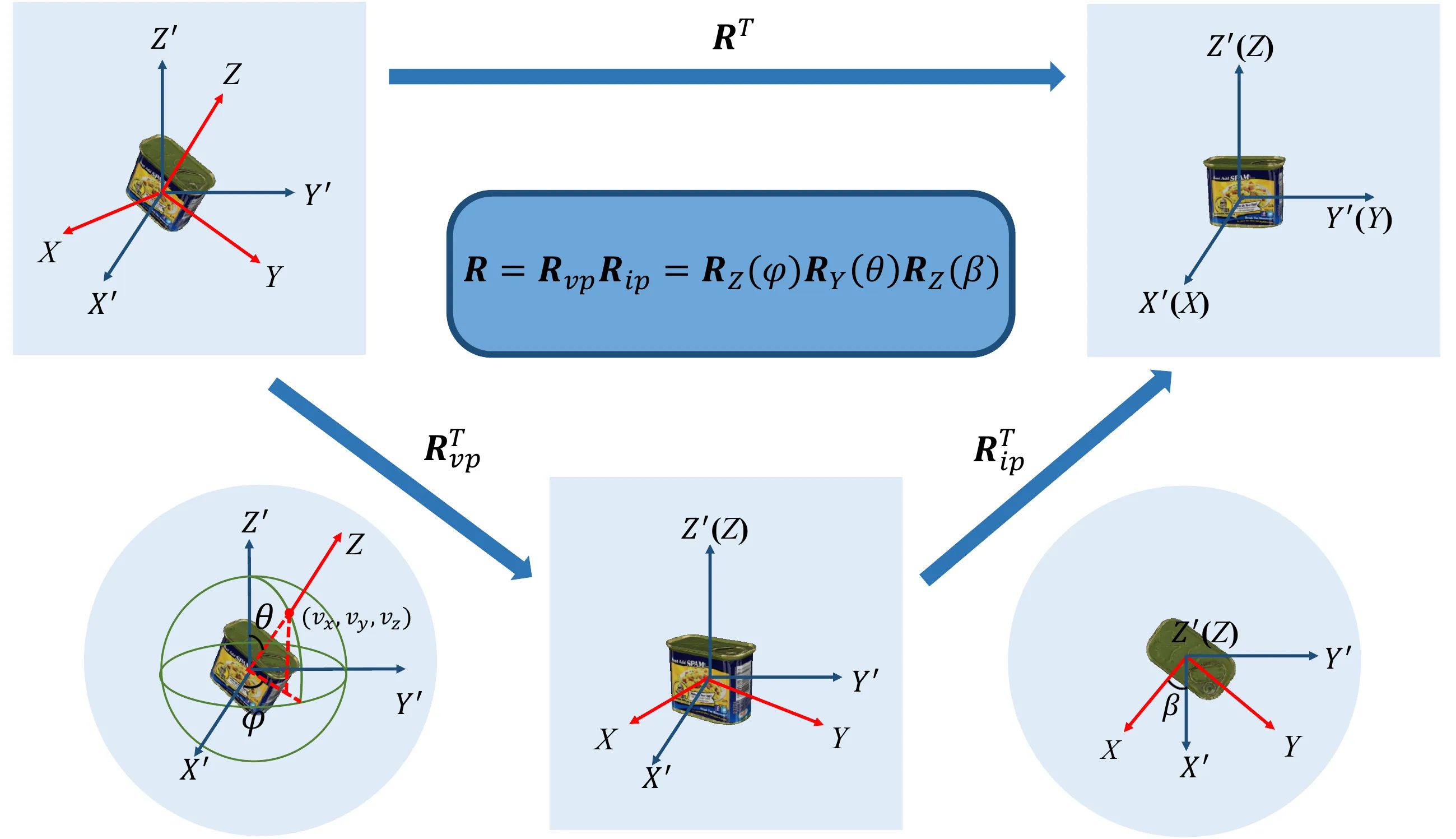
如图1所示，使用\(\mathbf{R}^T\)将物体坐标系XYZ与相机坐标系X'Y'Z'对齐（假设物体坐标系的XYZ的原点和相机坐标系的X'Y'Z'的原点重合），这个过程可以分为两步：

1. 第一步是将Z'轴与Z轴对齐，这一步由旋转矩阵\(\mathbf{R}_{vp}^T\)实现，“vp”代表的是“viewpoint”，即视角；
2. 第二步是将X'轴和Y'轴旋转到X轴和Y轴，这一步由旋转矩阵\(\mathbf{R}_{ip}^T\)实现，“ip”代表的是“in-plane”，即平面内。

那么将物体坐标系XYZ与相机坐标系X'Y'Z'对齐的过程可以表示为：\(\mathbf{R}^T = \mathbf{R}_{ip}^T\mathbf{R}_{vp}^T\)。

由于在\(SO(3)\)中，矩阵的转置就是矩阵的逆，那么将物体坐标系XYZ和相机坐标系X'Y'Z'恢复到原来的相对位置的过程可以表示为：

\[ \begin{equation}\label{eq1} \mathbf{R} = \mathbf{R}_{vp}\mathbf{R}_{ip}, \end{equation} \]

现在从物体坐标系XYZ和相机坐标系X'Y'Z'对齐时的状态出发，假设在物体坐标系Z轴上有一点\((0, 0, 1)\)，使用\(\mathbf{R} = \mathbf{R}_{vp}\mathbf{R}_{ip}\)的过程恢复到原来的相对位置，同样也分为两步：

1. 首先使用\(\mathbf{R}_{ip}\)让物体坐标系XYZ旋转绕Z'轴旋转\(\beta \in [0, 2\pi]\)，其旋转矩阵为：

   \[ \begin{equation}\label{eq2} \mathbf{R}_{ip} = \begin{bmatrix} \cos\beta & -\sin\beta & 0 \\ \sin\beta & \cos\beta & 0 \\ 0 & 0 & 1 \end{bmatrix}. \end{equation} \]

2. 此时，物体坐标系XYZ与相机坐标系X'Y'Z'不完全重合（Z轴与Z'轴是重合的，但X轴与X'轴、Y轴与Y'轴不重合），先将物体绕着Y'轴旋转\(\theta \in [0, \pi]\)，其旋转矩阵为：

   \[ \mathbf{R}_Y(\theta) = \begin{bmatrix} \cos\theta & 0 & \sin\theta \\ 0 & 1 & 0 \\ -\sin\theta & 0 & \cos\theta \end{bmatrix}; \]

3. 再将物体绕着Z'轴旋转\(\varphi \in [0, 2\pi]\)，其旋转矩阵为：

   \[ \mathbf{R}_Z(\varphi) = \begin{bmatrix} \cos\varphi & -\sin\varphi & 0 \\ \sin\varphi & \cos\varphi & 0 \\ 0 & 0 & 1 \end{bmatrix}; \]

那么结合上面的第2步和第3步，Z轴上的这一点的坐标变为\((v_x, v_y, v_z)\)，那么可以计算\((r, \varphi, \theta)\)为（这里我不理解，我觉得公式是错的）：

\[ \begin{equation}\label{eq3} \left\{\begin{matrix} \begin{aligned} r &= 1 \\ \varphi &= \arctan(\frac{v_x}{v_z}) \\ \theta &= \arccos(\frac{v_y}{r}) \end{aligned} \end{matrix}\right., \end{equation} \]

结合\(\mathbf{R}_Y(\theta)\)和\(\mathbf{R}_Z(\varphi)\)，可以得到：

\[ \begin{equation}\label{eq4} \begin{aligned} \mathbf{R}_{vp} &= \mathbf{R}_Z(\varphi)\mathbf{R}_Y(\theta) \\ &= \begin{bmatrix} \cos\varphi & -\sin\varphi & 0 \\ \sin\varphi & \cos\varphi & 0 \\ 0 & 0 & 1 \end{bmatrix} \begin{bmatrix} \cos\theta & 0 & \sin\theta \\ 0 & 1 & 0 \\ -\sin\theta & 0 & \cos\theta \end{bmatrix} \end{aligned}. \end{equation} \]

结合\(\eqref{eq4}\)和\(\eqref{eq2}\)，可以发现\(\mathbf{R} = \mathbf{R}_{vp}\mathbf{R}_{ip}\)与ZYZ欧拉角\(\varphi, \theta, \beta\)的参数化一致。

根据以上推导，估计物体的旋转可以分解为两个步骤：

1. 在球体上搜索点\((v_x, v_y, v_z)\)，以获得\(\varphi\)和\(\theta\)，共同得到视角旋转\(\mathbf{R}_{vp}\)；
2. 通过\(\mathbf{R}_{vp}\)将Z'轴与Z轴对齐，然后回归面内旋转\(\mathbf{R}_{ip}\)。

4. VI-Net for Rotation Estimation

4.1. Conversion as Spherical Representations

给定一个点集\(\mathcal{P} \in \mathbb{R}^{N \times 3}\)，每一个点都对应一个特征\(\mathcal{F} \in \mathbb{R}^{N \times C_0}\)（比如径向距离、RGB值、表面法线等），首先使用“Learning SO(3) Equivariant Representations with Spherical CNNs”和“DualPoseNet: Category-level 6D Object Pose and Size Estimation Using Dual Pose Network with Refined Learning of Pose Consistency”中的方法，生成在球体上定义的特征图\(\mathcal{S}_0 \in \mathbb{R}^{C_0 \times H_0 \times W_0}\)，其中\(N\)是点的数量，\(H_0 \times W_0\)是球面采样分辨率，\(C_0\)是特征维度（比如\(C_0 = 1\)为径向距离，\(C_0 = 3\)为RGB值或表面法线）。

Figure 3. An illustration of the feature padding in SPA-SConv. Best view in the electronic version.

具体来说，将球面坐标系沿方位轴（水平方向）和倾角轴（竖直方向）均匀的划分为\(H_0 \times W_0\)个网格（如图3所示），在每一个网格中，我们搜索径向距离最大的点，表示为\(\mathbf{p}_{h, w}^{max}\)，并让\(\mathcal{S}_0(h, w) = \mathbf{f}_{h, w}^{max} \in \mathcal{F}\)，对应于\(\mathbf{p}_{h, w}^{max}\)；如果这个区域内没有点，则让\(\mathcal{S}_0(h, w) = \mathbf{0}\)。

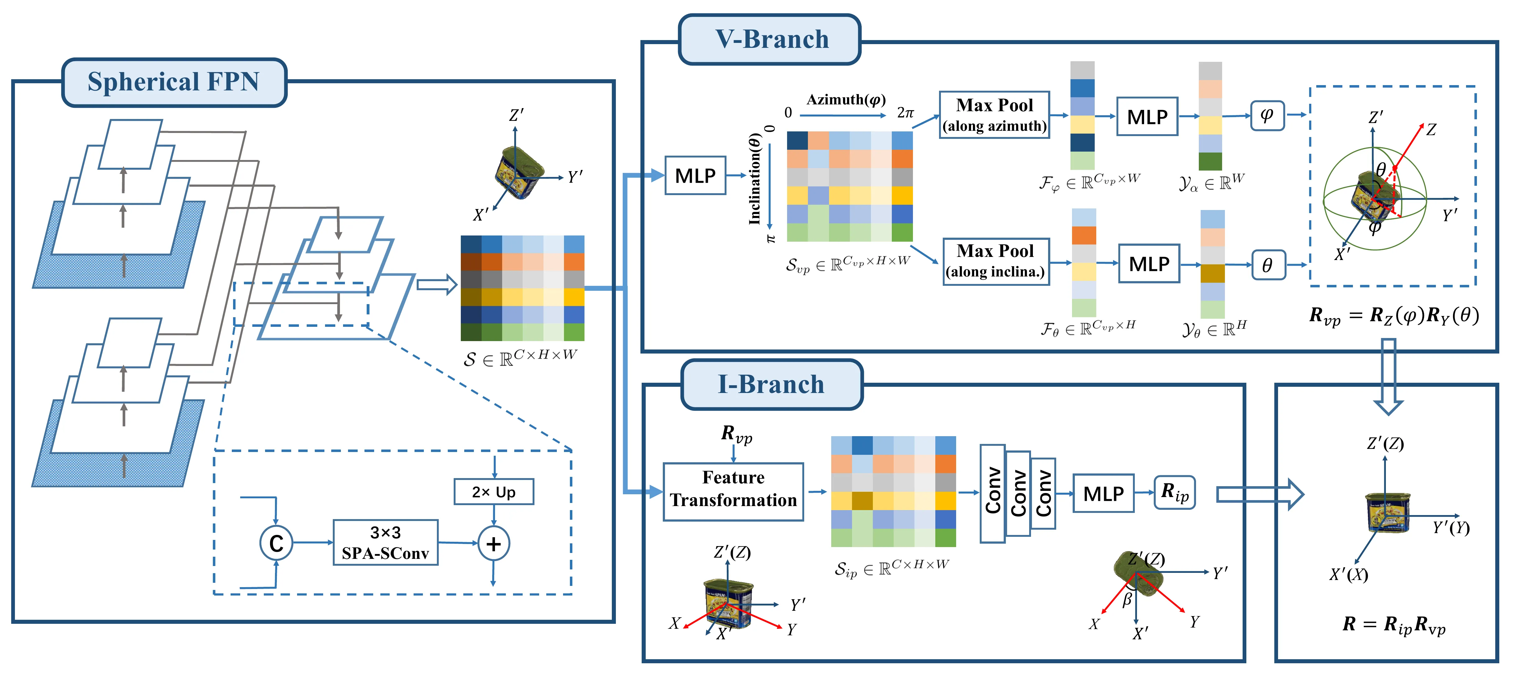
4.2. Spherical Feature Pyramid Network

使用ResNet18构建特征金字塔网络（FPN），用SPAtial Spherical Convolutions (SPA-SConvs)，代替传统的2D卷积，得到高级语义球形特征图\(\mathcal{S} \in \mathbb{R}^{C \times H \times W}\)，如图2所示。第5部分中会有详细介绍。

4.3. V-Branch

V-Branch估计视角旋转\(\mathbf{R}_{vp}\)，视角旋转中包含了方位角\(\varphi\)和倾角\(\theta\)，为了简化任务，可以分别估计\(\varphi\)和\(\theta\)，这也有效缓解了正负样本对不平衡的问题。图2给出了V-Branch的图示。

以两层MLP提升\(\mathcal{S}\)的特征维度，得到\(\mathcal{S}_{vp} \in \mathbb{R}^{C_{vp} \times H \times W}\)。为了学习水平方位角\(\varphi\)，在竖直方向上的倾角维度对\(S_{vp}\)进行最大池化，得到\(\mathcal{F}_\varphi \in \mathbb{R}^{C_{vp} \times W}\)，再将其送入另一个MLP中得到\(W\)方位角区域的概率图\(\mathcal{Y}_\alpha \in \mathbb{R}^W\)。\(\mathcal{Y}_\alpha\)中的每一个元素都表示该区域成为目标的可能性。将具有最大概率的元素的索引表示为\(w_{max}\)，则有：

\[ \begin{equation}\label{eq5} \varphi = \frac{w_{max} + 0.5}{W} \times 2\pi. \end{equation} \]

同样，对于倾角\(\theta\)，沿水平方向上的方位角维度对\(S_{vp}\)进行最大池化，得到\(\mathcal{F}_\theta \in \mathbb{R}^{C_{vp} \times H}\)，然后得到\(\mathcal{Y}_\beta \in \mathbb{R}^H\)，那么\(\theta\)可以计算如下：

\[ \begin{equation}\label{eq6} \theta = \frac{h_{max} + 0.5}{H} \times \pi. \end{equation} \]

其中\(h_{max}\)是\(\mathcal{Y}_\beta\)中最大概率的索引。最后，结合\(\eqref{eq5}\)、\(\eqref{eq6}\)和\(\eqref{eq4}\)，可以得到视角旋转\(\mathbf{R}_{vp} = \mathbf{R}_Z(\varphi)\mathbf{R}_Y(\theta)\)。

4.4. I-Branch

在V-Branch之后，我们已经得到了视角旋转\(\mathbf{R}_{vp}\)，那么就可以使用\(\mathbf{R}_{vp}\)将Z'轴与Z轴对齐（如图1所示）。对齐后可以构建一个新的球面特征图\(S_{ip} \in \mathbb{R}^{C \times H \times W}\)。\(\mathcal{S}\)的视点不变性使得在特征空间中实现变换以获得\(S_{ip}\)成为可能。

对于分辨率为\(H \times W\)的规则球面映射，我们将所有\(HW\)离散锚点的中心点表示为点集\(\mathcal{G} = \{\mathbf{g}\}\)。当我们用\(\mathbf{R}_{vp}\)将点集\(\mathcal{P} = \{\mathbf{p}\}\)旋转到\(\mathcal{P}^\prime = \{\mathbf{p}^\prime\} = \{\mathbf{R}_{vp}^T\mathbf{p}\}\)时，\(\mathcal{S}\)的锚点也旋转为\(\mathcal{G}^\prime = \{\mathbf{g}^\prime\} = \{\mathbf{R}_{vp}^T\mathbf{g}\}\)；我们将\(\mathbf{g}^\prime\)的特征标记为\(\mathcal{S}^{\mathbf{g}^\prime}\)。

为了从顶部观察物体，需要为变换后的\(\mathcal{P}^\prime\)构建一个新的球形特征图\(\mathcal{S}_{ip}\)。对于\(\mathcal{S}_{ip}\)，我们使用“PointNet++: Deep Hierarchical Feature Learning on Point Sets in a Metric Space”中的点特征加权插值方法，在每个锚点\(\mathbf{g}\)上生成其特征，表示为\(\mathcal{S}_{ip}^\mathbf{g}\)，如下所示：

\[ \begin{equation}\label{eq7} \mathcal{S}_{ip}^\mathbf{g} = \frac{\sum_{i = 1}^k a_i \mathcal{S}^{\mathbf{g}^\prime_i}}{\sum_{i = 1}^k a_i}, \end{equation} \]

其中\(a_i = \frac{1}{\Vert\mathbf{g} - \mathbf{g}^\prime_i\Vert}\)是按点距离衡量的插值权重，\(\{\mathbf{g}_i^\prime\}_{i = 1}^k \subset \mathcal{G}^\prime\)是\(\mathbf{g}\)的\(k\)个最近邻。

通过\(\eqref{eq7}\)实现从\(\mathcal{S}\)到\(\mathcal{S}_{ip}\)的转换后，使用卷积来降低\(\mathcal{S}_{ip}\)的分辨率，并为\(\mathbf{R}_{ip}\)的回归提取一个全局特征图，如图2所示。旋转的连续6D表示作为回归的输出，然后转换为旋转矩阵\(\mathbf{R}_{ip}\)。这里预测的\(\mathbf{R}_{ip}\)并不只包含面内旋转，而是残差视点旋转和精确面内旋转的组合。

4.5. Training of VI-Net

对于V-Branch，使用来自“Focal Loss for Dense Object Detection”的焦点损失，给定GT \(\hat{\mathcal{Y}}_\varphi \in \mathbb{R}^W\)和\(\hat{\mathcal{Y}}_\theta \in \mathbb{R}^H\)，损失函数为：

\[ \begin{equation}\label{eq8} \mathcal{L}_{vp} = \mathcal{D}_{FL}(\mathcal{Y}_\varphi, \hat{\mathcal{Y}}_\varphi) + \mathcal{D}_{FL}(\mathcal{Y}_\theta, \hat{\mathcal{Y}}_\theta), \end{equation} \]

其中：

\[ \begin{equation}\label{eq9} \mathcal{D}_{FL}(\mathcal{Y}, \hat{\mathcal{Y}}) = \frac{1}{M} \sum_{i = 1}^M -\alpha(1 - t_{i, t})^\gamma \log(y_{i, t}), \end{equation} \]

且：

\[ \begin{equation}\label{eq10} y_{i, t} = \begin{cases} y_i, & \text{if} & \hat{y}_i = 1 \\ 1 - y_i, & \text{if} & \hat{y}_i = 0 \end{cases}, \end{equation} \]

其中\(\mathcal{Y} = \{y_i\}_{i = 1}^M\)，\(\hat{\mathcal{Y}} = \{\hat{y}_i \in \{0, 1\}\}_{i = 1}^M\)。\(\alpha\)是权重因子，\(\gamma\)表示调节因子的指数。

给定GT \(\hat{\mathbf{R}}\)，我们对I-Branch的输出\(\mathbf{R} = \mathbf{R}_{vp}\mathbf{R}_{ip}\)监督如下：

\[ \begin{equation}\label{eq11} \mathcal{L}_{ip} = \Vert\mathbf{R} - \hat{\mathbf{R}}\Vert = \Vert\mathbf{R}_{vp}\mathbf{R}_{ip} - \hat{\mathbf{R}}\Vert. \end{equation} \]

结合\(\eqref{eq8}\)和\(\eqref{eq11}\)，VI-Net的训练目标为：

\[ \begin{equation}\label{eq12} \min \mathcal{L} = \mathcal{L}_{ip} + \lambda \mathcal{L}_{vp}. \end{equation} \]

其中\(\lambda\)是平衡两个损失的权重因子。

5. Spatial Spherical Convolution

方法建立具有规则2D空间大小的球形特征图以实现旋转估计，特征图建立后，就可以使用传统的2D卷积来处理球形信号。但是，直接在球形特征图上使用2D卷积会有边界问题，比如特征图\(S_0\)上的\(S_0(h, 1)\)和\(S_0(h, W)\)在球面上是相连的，而在特征图中则有很大的距离。此外，为了支持I-Branch中的特征转换以便从天顶方向查看，backbone中的卷积也需要是视角一致的。这里提出了SPAtial Spherical Convolution，即SPA-SConv，在球面上连续提取视角一致的特征，可以灵活的适应现有的卷积架构，例如4.2节中的FPN。

给定输入球面特征图\(\mathcal{S}_l \in \mathbb{R}^{C_l \times H_l \times W_l}\)和卷积参数（如卷积核大小\(K\)、步长\(s\)和输出通道数\(C_{l + 1}\)等），我们分两步实现SPA-SConv：

1. 将\(\mathcal{S}_l\)padding到\(S_l^{pad} \in \mathbb{R}^{C_l \times (H_l + 2P) \times (W_l + 2P)}\)，其中\(P = \frac{K - 1}{2}\)；
2. 将对称卷积应用于\(S_l^{pad}\)，基于没有padding的常规2D卷积，得到输出球面特征图\(\mathcal{S}_{l + 1} \in \mathbb{R}^{C_{l + 1} \times H_{l + 1} \times W_{l + 1}}\)，其中\(H_{l + 1} = \lfloor\frac{H_l}{s}\rfloor\)，\(W_{l + 1} = \lfloor\frac{W_l}{s}\rfloor\)（为简单起见，我们假设2D卷积核的长度和宽度都是\(K\)，\(K\)是一个奇数）。

图3可视化了从\(\mathcal{S}_l\)到\(S_l^{pad}\)的padding过程。首先，将\(\mathcal{S}_l\)的中心作为\(\mathcal{S}_l^{pad}\)的中心：

\[ \begin{equation}\label{eq13} S_l^{pad}(h + P, w + P) = \mathcal{S}_l(h, w), \end{equation} \]

对于\(\forall h = 1, 2, \cdots, H_l\)和\(\forall w = 1, 2, \cdots, W_l\)。接下来，我们沿倾角方向填充\(\mathcal{S}_l\)：

\[ \begin{equation}\label{eq14} \begin{aligned} S_l^{pad}(p, w + P) &= \mathcal{S}_l^{pad}(2P - p + 1, w^\prime), \\ \text{and } S_l^{pad}(H_l + P + p, w + P) &= \mathcal{S}_l^{pad}(H_l + P - p + 1, w^\prime), \end{aligned} \end{equation} \]

其中：

\[ \begin{equation}\label{eq15} w^\prime = \begin{cases} w + \frac{W_l}{2} + P & \text{if} & w \le \frac{W_l}{2} \\ w - \frac{W_l}{2} + P & & \text{otherwise} \end{cases}, \end{equation} \]

对于\(\forall p = 1, 2, \cdots, P\)和\(\forall w = 1, 2, \cdots, W_l\)。最后，我们沿方位角方向填充\(\mathcal{S}_l\)：

\[ \begin{equation}\label{eq16} \begin{aligned} S_l^{pad}(h, p) &= \mathcal{S}_l^{pad}(h, W_l + p), \\ \text{and } S_l^{pad}(h, W_l + P + p) &= \mathcal{S}_l^{pad}(h, P + p), \end{aligned}, \end{equation} \]

对于\(\forall p = 1, 2, \cdots, P\)和\(\forall w = 1, 2, \cdots, W_l\)。

得到\(S_l^{pad}\)后，我们就可以使用2D卷积来实现视点一致的对称卷积运算：

\[ \begin{equation}\label{eq17} \mathcal{S}_{l + 1} = \text{Max}(\text{Conv}(\mathcal{S}_l^{pad}; \kappa_l), \text{Conv}(\mathcal{S}_l^{pad}, \text{Flip}(\kappa_l))), \end{equation} \]

其中，\(\text{Conv}\)表示2D卷积、\(\text{Flip}\)表示卷积核的水平翻转、\(\text{Max}\)表示元素级最大池化。根据“PointNet: Deep Learning on Point Sets for 3D Classification and Segmentation”中的方法，\(\text{Max}\)作为对称函数来聚合特征，并保持视点一致的性质，补充材料中给出了此特性的证明。

6. Category-level 6D Object Pose Estimation

VI-Net估计\(\mathbf{R}, \mathbf{t}, \mathbf{s}\)，且在推理时CAD模型不可用。给定一张RGBD图，首先使用MaskRCNN分割物体，对于每个裁剪出的具有点集\(\mathcal{P} = \{\mathbf{p}\}\)的物体，首先使用PointNet++估计\(\mathbf{t}\)和\(\mathbf{s}\)，然后在旋转估计时，将估计出的\(\mathbf{t}\)和\(\mathbf{s}\)作为初始化输入到VI-Net中进行归一化：\(\mathcal{P}^\prime = \{\frac{\mathbf{p} - \mathbf{t}}{\Vert\mathbf{s}\Vert}\}\)，最后使用VI-Net估计\(\mathbf{R}\)。

6.1. Experimental Setups

6.2. Comparisons with Existing Methods

Table 1. Quantitative comparisons of different methods for category-level 6D object pose estimation on REAL275 and CAMERA25 datasets [31]. Overall best results are in bold and the second best results are underlined. '∗' denotes the IoU metrics used in [23] rather than those in [31].

Method	Use of Shape Priors	REAL275					CAMERA25
		IoU75∗	5°2cm	5°5cm	10°2cm	10°5cm	IoU75∗	5°2cm	5°5cm	10°2cm	10°5cm
NOCS [31]	✕	9.4	7.2	10.0	13.8	25.2	37.0	32.3	40.9	48.2	64.6
FS-Net [5]	✕	-	-	28.2	-	60.8	-	-	-	-	-
DualPoseNet [20]	✕	30.8	29.3	35.9	50.0	66.8	71.7	64.7	70.7	77.2	84.7
GPV-Pose [8]	✕	-	32.0	42.9	-	73.3	-	72.1	79.1	-	89.0
SS-ConvNet [18]	✕	-	36.6	43.4	52.6	63.5	-	-	-	-	-
PN2 + VI-Net (Ours)	✕	48.3	50.0	57.6	70.8	82.1	79.1	74.1	81.4	79.3	87.3
SPD [28]	✓	27.0	19.3	21.4	43.2	54.1	46.9	54.3	59.0	73.3	81.5
CR-Net [32]	✓	33.2	27.8	34.3	47.2	60.8	75.0	72.0	76.4	81.0	87.7
CenterSnap-R [14]	✓	-	-	29.1	-	64.3	-	-	66.2	-	81.3
ACR-Pose [10]	✓	-	31.6	36.9	54.8	65.9	-	70.4	74.1	82.6	87.8
SAR-Net [17]	✓	-	31.6	42.3	50.3	68.3	-	66.7	70.9	75.3	80.3
SSP-Pose [37]	✓	-	34.7	44.6	-	77.8	-	64.7	75.5	-	87.4
SGPA [4]	✓	37.1	35.9	39.6	61.3	70.7	69.1	70.7	74.5	82.7	88.4
RBP-Pose [36]	✓	-	38.2	48.1	63.1	79.2	-	73.5	79.6	82.1	89.5
SPD + CATRE [23]	✓	43.6	45.8	54.4	61.4	73.1	76.1	75.4	80.3	83.3	89.3
DPDN [19]	✓	-	46.0	50.7	70.4	78.4	-	-	-	-	-

Figure 4. Qualitative comparisons between the state-of-the-art method of DPDN [19] and our proposed one on REAL275 dataset [31].

Figure 5. Plottings of per-category average precision versus different rotation/translation error thresholds for our proposed method on REAL275 dataset [31].

6.3. Ablation Studies and Analyses

Table 2. Ablation studies of the variants of our VI-Net with or without rotation decomposition (R.D.) on REAL275 dataset [31].

	R.D.	5°2cm	5°5cm
Baseline1: Avg Pool + MLP	✕	45.0	51.8
Baseline2: Flattening + MLP	✕	42.7	48.8
VI-Net	✓	50.0	57.6

Table 3. Ablation studies of the variants of the V-Branch and I-Branch in our VI-Net on REAL275 dataset [31].

Variants of V-Branch	Feature Trans. in I-Branch	5°2cm	5°5cm	10°2cm	10°5cm
Direct Regression	✕	26.3	28.9	54.1	61.1
Binary Classification (1-branch)	✕	30.8	34.4	65.5	75.3
Binary Classification (2-branch)	✕	33.7	37.9	65.4	75.4
Direct Regression	✓	43.1	48.3	68.0	78.1
Binary Classification (1-branch)	✓	49.3	56.9	69.4	79.7
Binary Classification (2-branch)	✓	50.0	57.6	70.8	82.1

Table 4. Quantitative comparisons of SPE-SConv [9] and variants of our proposed SPA-SConv on REAL275 dataset [31].

Type of Convolution	Padding	Symmetric Operation	5°2cm	5°5cm
SPE-SConv [9]	-	-	35.1	40.8
SPA-SConv	✕	✕	46.9	53.2
	✕	✓	48.5	55.5
	✓	✓	50.0	57.6

Table 5. Quantitative comparisons between VI-Net+ts and PN2 for translation and size estimation on REAL275 dataset [31].

	5°2cm	5°5cm	10°2cm	10°5cm
VI-Net+ts	45.0	56.0	65.9	80.5
PN2 + VI-Net	50.0	57.6	70.8	82.1

Table 6. Quantitative comparisons of different input data types of VI-Net on REAL275 dataset [31].

Data Type	5°2cm	5°5cm	10°2cm	10°5cm
Depth	43.0	52.1	64.3	77.0
RGB + Depth	50.0	57.6	70.8	82.1

Figure 6. Qualitative results of the predicted viewpoint rotation \(\mathbf{R}_{vp}\) from V-Branch and the final output rotation \(\mathbf{R}\) from VI-Net.

7. Conclusion