【论文笔记】Co-op: Correspondence-based Novel Object Pose Estimation
Co-op: Correspondence-based Novel Object Pose Estimation
| 方法 | 类型 | 训练输入 | 推理输入 | 输出 | pipeline |
|---|---|---|---|---|---|
| Co-op | 任意级 | RGB + CAD | RGB + CAD | 绝对\(\mathbf{R}, \mathbf{t}\) |
- 2025.04.06:使用patch-patch的匹配来确定与查询最接近的模板并得到2D-3D的匹配,然后使用EPnP计算粗略位姿。在优化时,将查询和模板之间的flow定义为一个单变量拉普拉斯分布,预测这个分布以优化位姿。
Abstract
1. Introduction
Our contributions can be summarized as follows:
- We present Co-op, a novel framework for unseen object pose estimation in RGB-only cases. Co-op does not require additional training or fine-tuning for new objects and outperforms existing methods by a large margin on the seven core datasets of the BOP Challenge.
- We propose a method for fast and accurate coarse pose estimation using a hybrid representation that combines patch-level classification and offset regression.
- Additionally, we propose a precise object pose refinement method. It estimates dense correspondences defined by probabilistic flow and learns confidence end-to-end through a differentiable PnP layer.
2. Related Work
3. Method
3.1. Coarse Pose Estimation
Template Generation:粗略位姿估计阶段使用和GigaPose类似的方法,生成仅包含面外旋转的模板来减少位姿估计需要的模板数。
使用“Templates for 3D Object Pose Estimation Revisited: Generalization to New Objects and Robustness to Occlusions”和“CNOS: A Strong Baseline for CAD-based Novel Object Segmentation”中的方法生成模板。
Hybrid Representation:Query图像和Template图像分别使用\(\mathcal{I}_Q, \mathcal{I}_T \in \mathbb{R}^{H \times W \times 3}\)表示。为了提高泛化性,使用了一种结合patch分类和偏移回归的混合表示。
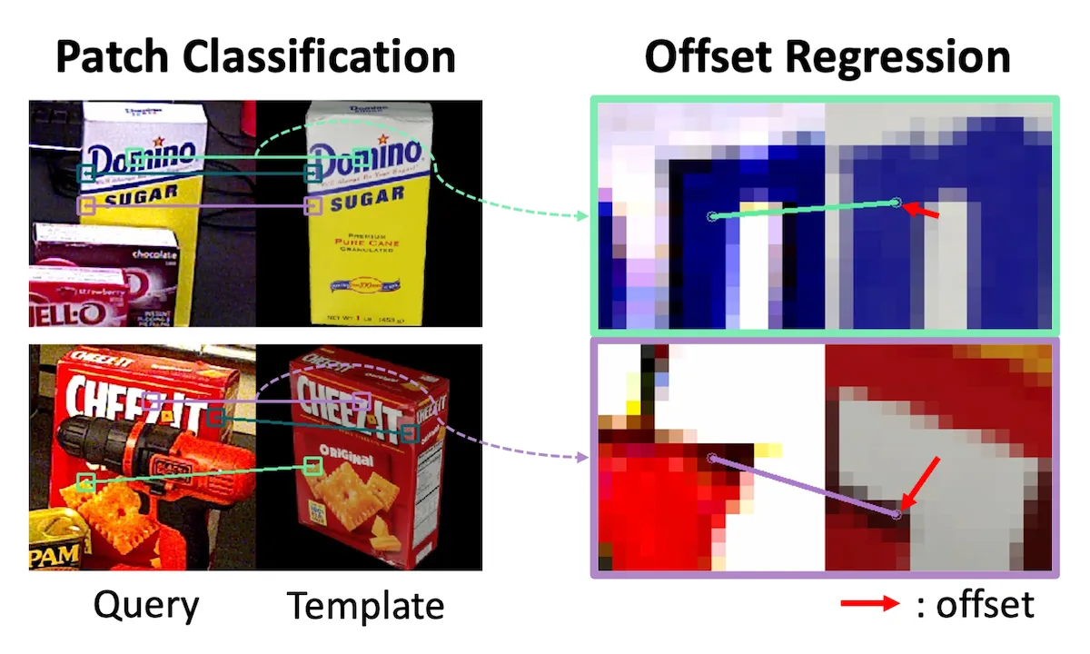
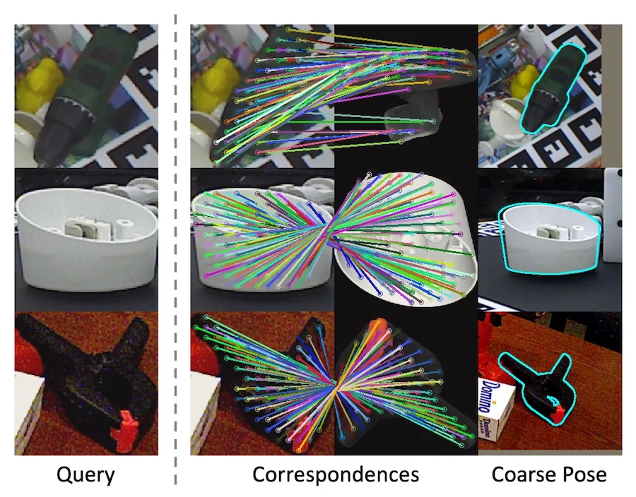
图3左侧是patch分类结果,右侧是偏移回归结果。
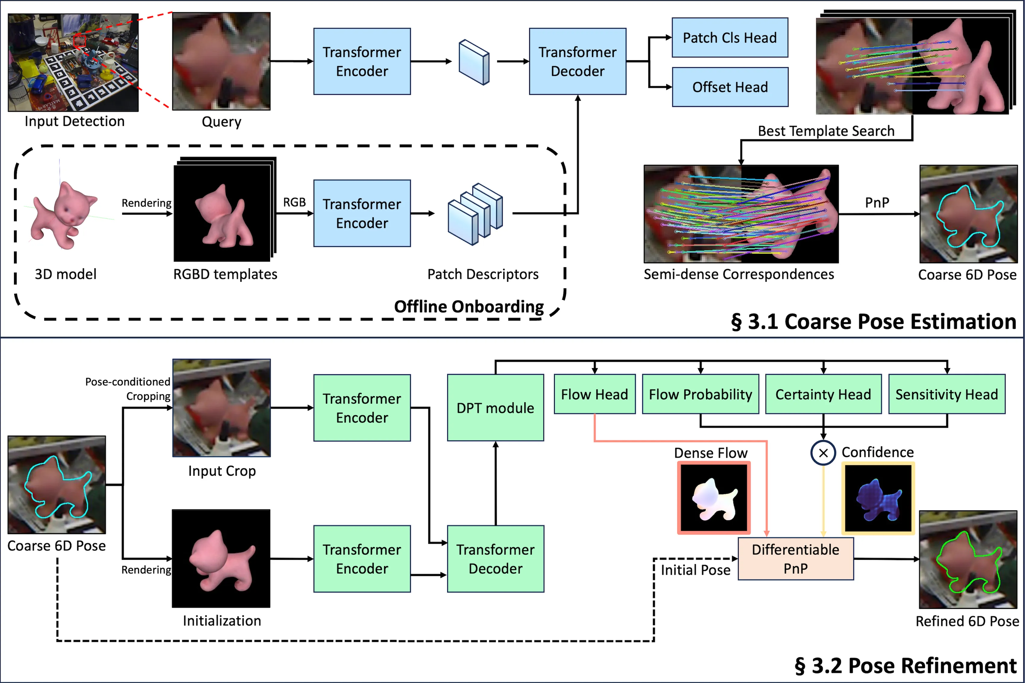
如图2所示,使用Transformer Encoder提取Query图像和Template图像的特征,然后使用Transformer Decoder生成patch分类结果和偏移回归结果。
Encoder将\(\mathcal{I}_Q\)和\(\mathcal{I}_T\)作为输入,提取特征图\(\mathcal{F}_Q, \mathcal{F}_T \in \mathbb{R}^{\frac{H}{16} \times \frac{W}{16} \times 1024}\)。然后Decoder和后续头处理\(\mathcal{F}_Q\)和\(\mathcal{F}_T\),计算patch级分类\(\mathcal{C} \in \mathbb{R}^{\frac{H}{16} \times \frac{W}{16} \times K}\)和xy-offsets \(\mathcal{U} \in \mathbb{R}^{\frac{H}{16} \times \frac{W}{16} \times 2}\)。
其中,\(K = \frac{H}{16} \times \frac{W}{16} + 1\)表示patch级分类的类数,\(\frac{H}{16} \times \frac{W}{16}\)为patch的数量,最后的\(+1\)表示没有匹配的情况,例如遮挡。对于特征图中的每个位置\((i, j)\),\(\mathcal{C}_{i, j} \in \mathbb{R}^K\)包含分类分数,指示Query \((i, j)\)位置上的patch和Template中\(\frac{H}{16} \times \frac{W}{16}\)个patch的匹配情况。
在此之后,我们将索引定义为\(c_{i, j} = \arg \max_{k \in 1, 2, \cdots, K} \mathcal{C}_{i, j}^k\),将偏移的范围定义在\(\mathcal{U}_{i, j} \in [-0.5, 0.5]\)。在\(c_{i, j} \ne K\)的位置\((i, j)\)上,可以使用下面的公式来计算Query中下标为\((i, j)\)的patch的中心点在Template patch中的对应点\(\mathcal{M}_{i, j}^T\):
\[ \begin{equation}\label{eq1} \mathcal{M}_{i, j}^T = \left(\begin{bmatrix} c_{i, j} \mod 16 + 0.5 \\ \lfloor \frac{c_{i, j}}{16} \rfloor + 0.5 \end{bmatrix} + \mathcal{U}_{i, j}\right) \times 16. \end{equation} \]
添加\(\mathcal{U}_{i, j}\)可优化特征图网格中的位置。乘16会将该位置映射回原始图像\(\mathcal{I}_Q\)和\(\mathcal{I}_T\)的坐标系,因为特征图中的每个位置都对应原始图像中一个大小为\(16 \times 16\)的patch。对应的Query图像位置\(\mathcal{M}_{i, j}^Q\)为\(((i + 0.5) \times 16, (j + 0.5) \times 16)\),即每个Query patch的中心位置。\(\mathcal{I}_Q\)和\(\mathcal{I}_T\)的对应关系定义为\(\mathcal{M}_{i, j} = (\mathcal{M}_{i, j}^Q, \mathcal{M}_{i, j}^T)\)。
Pose Fitting:我们计算\(\mathcal{I}_Q\)和所有\(\mathcal{I}_T\)的对应关系\(\mathcal{M}\),并选择与Query最相似的模板\(k\)。每个模板的相似性得分定义如下:
\[ \begin{equation}\label{eq2} S_t = \sum_{i, j} \begin{cases} \max(\mathcal{C}_{i, j}), & \text{if } c_{i, j} \ne K \\ 0, & \text{otherwise} \end{cases}. \end{equation} \]
如果\(c_{i, j} = K\)(表示遮挡或不匹配的patch),我们从总和中排除\(\max(\mathcal{C}_{i, j})\)。通过计算每个模板的\(S_t\),我们选择相似度得分最高的模板作为\(\mathcal{I}_Q\)的最佳匹配,然后基于模板中的深度信息构建2D-3D的对应关系,然后使用RANSAC和EPnP来计算初始位姿。
3.2. Pose Refinement
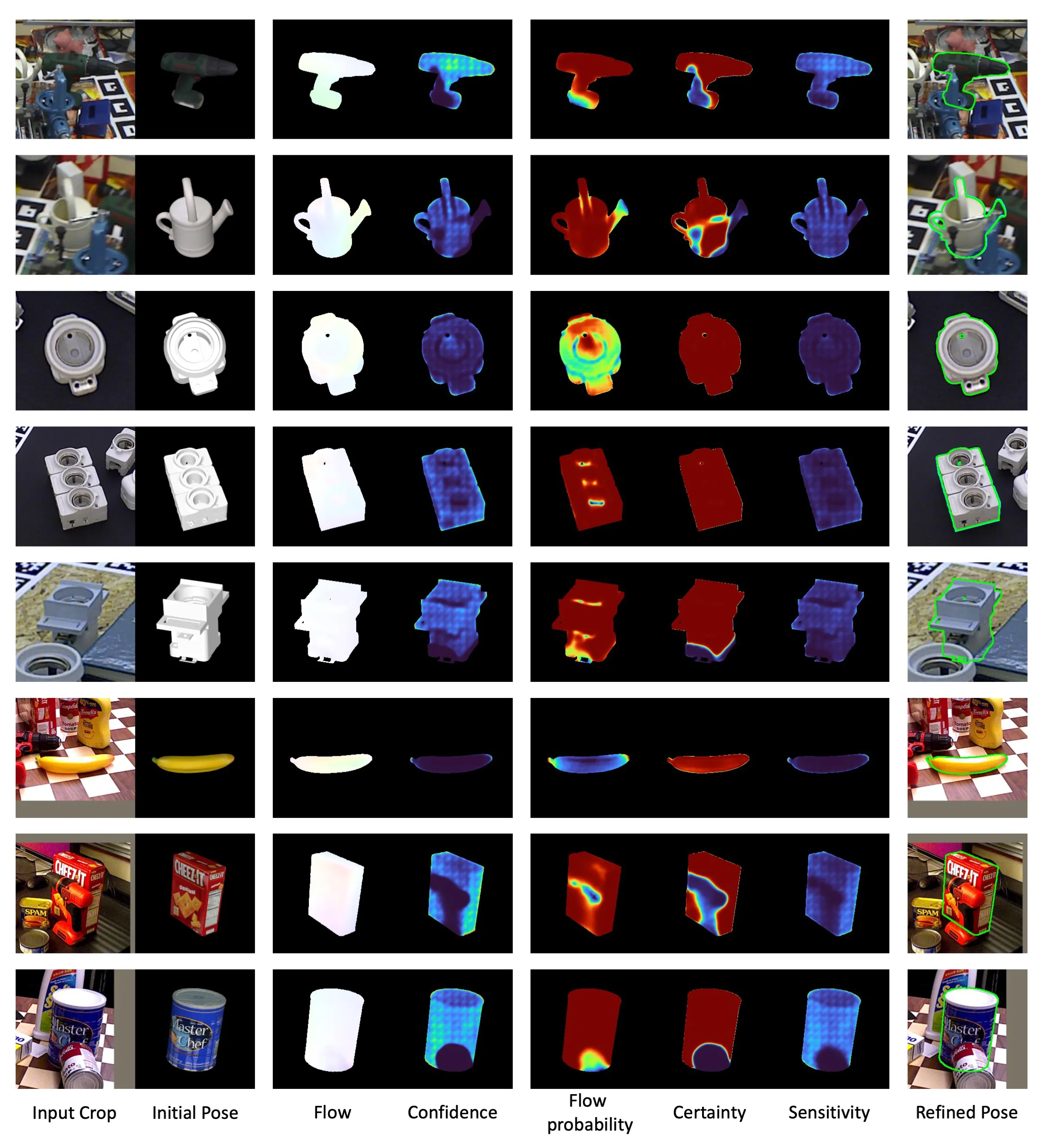
如图2所示,细化模型就是在粗略位姿估计模型的基础上增加一个密集预测Transformer(DPT)。DPT支持像素级预测,从而实现精确的位姿优化。此外,使用渲染-比较方法迭代优化位姿,该阶段克服了在粗略位姿估计阶段使用预渲染模板所带来的限制,比如自遮挡。
Probabilistic Flow Regression:与“Perspective Flow Aggregation for Data-Limited 6D Object Pose Estimation”和“GenFlow: Generalizable Recurrent Flow for 6D Pose Refinement of Novel Objects”类似,细化模型估计Query \(\mathcal{I}_T\)和Render \(\mathcal{I}_R\)之间的流动以优化位姿。要从流中准确恢复位姿,必须防止不准确的流显著影响位姿计算。所以,“Perspective Flow Aggregation for Data-Limited 6D Object Pose Estimation”使用RANSAC从位姿估计中概率的排除不准确的流。但是,由于RANSAC对异常值分布敏感,因此当异常值普遍存在或分布不均匀时,RANSAC的性能会下降。
与之前基于流的细化方法不同,我们的目标是学习流的条件概率。根据“ASpanFormer: Detector-Free Image Matching with Adaptive Span Transformer”和“PDC-Net+: Enhanced Probabilistic Dense Correspondence Network”,我们将这个条件概率定义为\(p(Y | \mathcal{I}_Q, \mathcal{I}_R; \theta)\),其中\(Y\)是\(\mathcal{I}_Q\)和\(\mathcal{I}_R\)之间的流,\(\theta\)是模型参数。很多方法通过学习预测\(Y\)的方差来实现这一点,并且使用高斯分布或拉普拉斯分布对预测密度进行建模。我们将其建模为单变量拉普拉斯分布以简化问题。具体来说,\(p(Y | \mathcal{I}_Q, \mathcal{I}_R; \theta)\)建模为均值为\(\mu \in \mathbb{R}^{H \times W \times 2}\),尺度为\(b \in \mathbb{R}^{H \times W \times 1}\)的拉普拉斯分布,两者均由网络预测。将流估计表示为概率回归,使我们的模型通过调整尺度参数\(b\)专注于高度可靠的对应关系。
Flow Confidence:要使用模型估计的流来计算位姿,我们需要置信度\(\mathcal{W} \in \mathbb{R}^{H \times W \times 1}\)。\(\mathcal{W}\)决定了在计算可微分PnP层中的位姿时,每个流误差的权重。\(\mathcal{W}\)是根据确定性、敏感性和流概率计算得出的,这些概率是通过不同的损失函数学习的。确定性估计从\(\mathcal{I}_R\)到\(\mathcal{I}_Q\)的流是否被遮挡。灵敏度是从位姿损失中学习的,并高亮具有丰富纹理或物体边缘的区域。与“PDC-Net+: Enhanced Probabilistic Dense Correspondence Network”类似,我们定义了流概率\(P_R\),它表示真实流动\(y\)位于平均光流\(\mu\)、半径为\(R\)范围内的概率。其计算方式如下:
\[ \begin{equation}\label{eq3} P_R = P(\Vert y - \mu\Vert_1 < R) = 1 - \exp\left(-\frac{R}{b}\right). \end{equation} \]
\(P_R\)是可靠性的可解释度量,表示阈值为\(R\)的流的准确性。流置信度\(\mathcal{W}\)计算为确定性、敏感性和\(P_R\)的元素乘积。这意味着在没有遮挡(高质量)、有判别信息可用于解决位姿(高灵敏度)以及准确性(高\(P_R\))时,\(\mathcal{W}\)将具有更高的值。
Pose Update:为了使用流\(Y\)和流置信度\(\mathcal{W}\)计算细化后的6D位姿\(\mathbf{P}_\text{refined}\),我们使用基于Levenberg-Marquardt(LM)的PnP求解器。给定输入位姿\(\mathbf{P}_\text{input} = [\mathbf{R}_\text{input} | \mathbf{t}_\text{input}]\),相机内参矩阵\(\mathbf{K}\)和对应于\(\mathcal{I}_R\)的深度图\(\mathcal{D}_R\),我们计算\(\mathcal{I}_R\)对应的3D空间坐标\(\mathbf{x}_{u, v}^\text{3D}\),如下所示:
\[ \begin{equation}\label{eq4} \mathbf{x}_{u, v}^\text{3D} = \mathbf{R}_\text{input}^{-1}(\mathbf{K}^{-1}\mathcal{D}_R(u, v)\mathbf{x}_{u, v}^\text{2D} - \mathbf{t}_\text{input}), \end{equation} \]
其中\((u, v)\)是\(\mathcal{I}_R\)中的像素坐标,\(\mathcal{D}_R(u, v)\)是每个像素的深度值,且\(\mathbf{x}_{u, v}^\text{2D} = (u, v, 1)^T\)。我们通过最小化加权重投影误差的平方和来优化6D位姿,如下所示:
\[ \begin{equation}\label{eq5} \underset{\mathbf{R}, \mathbf{t}}{\arg\min}\frac{1}{2}\sum_u\sum_v\Vert\mathcal{W}(u, v) \times (\pi(\mathbf{R}\mathbf{x}_{u, v}^\text{3D} + \mathbf{t}) - ((u, v)^T + Y(u, v)))\Vert^2. \end{equation} \]
其中,\(\pi\)是重投影函数,它使用相机内参\(\mathbf{K}\)将相机坐标中的3D点映射到2D图像点。
根据之前的工作“GenFlow: Generalizable Recurrent Flow for 6D Pose Refinement of Novel Objects”,我们使用LM算法分三次迭代更新位姿,并使用Gauss-Newton算法进一步将其细化为最终位姿。
3.3. Pose Selection
在粗略位姿估计阶段,最佳评分模板可能无法提供用于细化的最佳初始位姿。例如,选择相对于GT旋转180度的模板(见图4)会使优化变得具有挑战性。
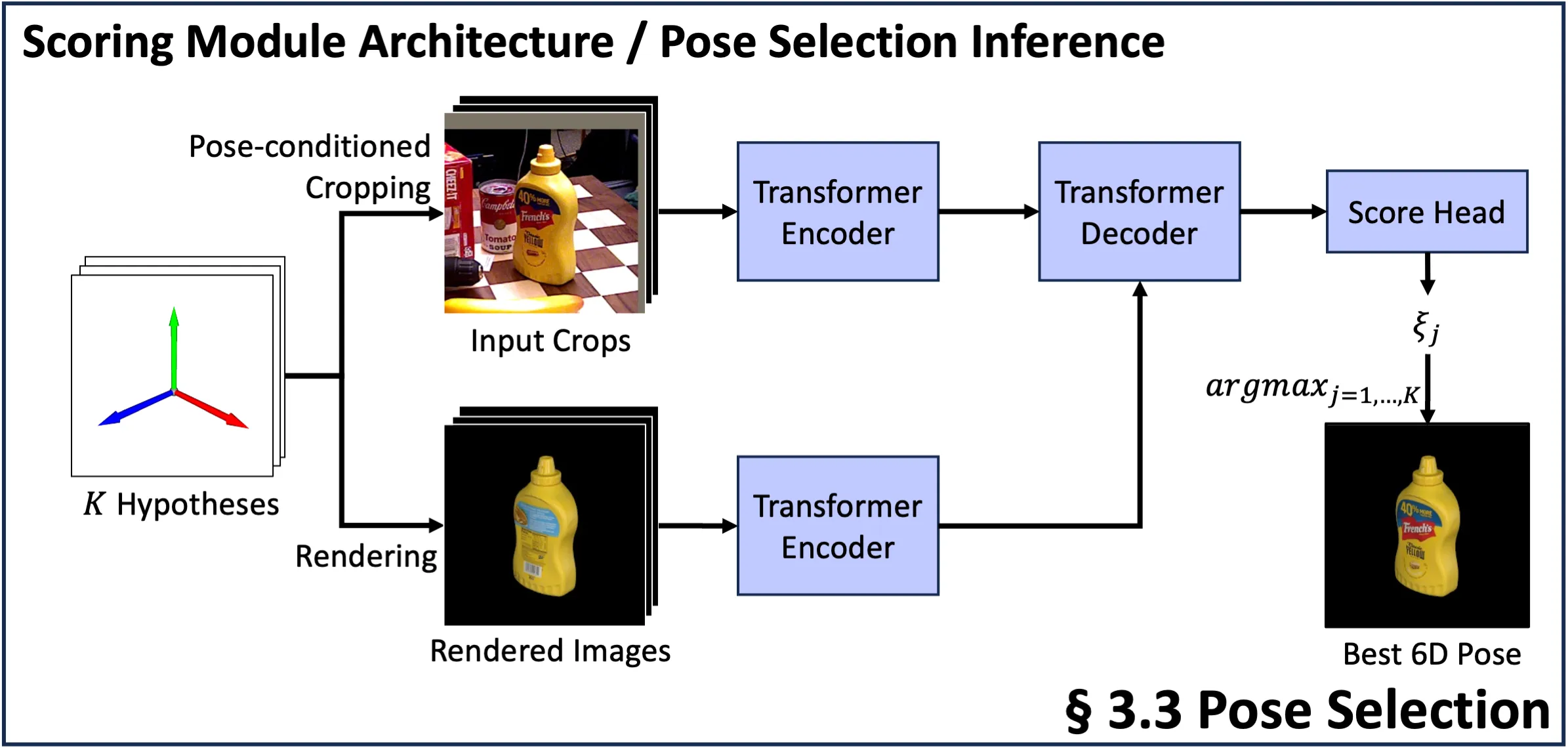
为了解决这个问题,“MegaPose”、“GenFlow”、“GigaPose”、“FoundPose”、“FoundationPose”等方法采用多重假设策略:生成\(N\)个粗略位姿估计,细化每个估计,并通过将渲染的结果和查询图像进行比较来选择最佳匹配。我们的位姿选择模型以查询图像和模板作为输入,在粗略位姿估计模型的基础上增加一个评分头来对每个位姿假设进行评分。即使这会增加推理时间,但是考虑多个优化位姿能够避免难以优化模板导致最终位姿较差的情况。
3.4. Training
Datasets:为了训练我们的三个模型(粗略位姿估计器、位姿优化器和位姿选择器),我们需要具有GT 6D位姿标注的RGBD图像。我们使用“MegaPose: 6D Pose Estimation of Novel Objects via Render & Compare”提供的大规模数据集。该数据集由使用“BlenderProc2: A Procedural Pipeline for Photorealistic Rendering”生成的合成数据组成,其中包含来自“ShapeNet: An Information-Rich 3D Model Repository”和“Google Scanned Objects: A High-Quality Dataset of 3D Scanned Household Items”的各种对象,包括全面的GT 6D位姿标注和对象掩码。
Coarse Model:我们的粗略位姿估计模型经过训练,用于估计查询图像\(\mathcal{I}_Q\)和模板图像\(\mathcal{I}_T\)之间的对应关系。和“GigaPose: Fast and Robust Novel Object Pose Estimation via One Correspondence”相似,我们选取的模板与围绕目标物体裁剪出的训练图像相比,具有相似的面外旋转角度,但面内旋转角度不同。如图5所示,我们的模型旨在估计查询图像和模板之间对于面内旋转具有不变性的对应关系。这种不变性意味着这些模板只需考虑面外旋转情况,从而大幅减少了所需模板的数量。由于我们拥有目标物体的3D模型,我们可以通过将3D模型投影到查询图像和模板图像的图像平面上,来生成这些对应关系。我们的模型经过训练就是为了估计这些生成的2D-2D的对应关系。
Refiner Model:我们的优化模型的训练方式与之前采用“渲染-比较”方法的研究工作如“CosyPose”、“MegaPose”、“GenFlow”等类似。我们通过向真实位姿\(\mathbf{P}_\text{gt}\)添加均值为0的高斯噪声来生成含噪声的输入位姿\(\mathbf{P}_\text{input}\),其中沿\(x\)、\(y\)、\(z\)轴的平移噪声标准差分别为\((0.01, 0.01, 0.05)\),并且在欧拉角中每个轴的旋转噪声标准差为15度。该模型经过训练,能够从\(\mathbf{P}_\text{input}\)中预测出\(\mathbf{P}_\text{gt}\)。
Selection Model:我们的选择模型经过训练,能够基于含噪输入姿态\(\mathbf{P}_\text{input}\)来评估查询图像\(\mathcal{I}_Q\)与参考图像\(\mathcal{I}_R\)之间的相似度,以便从多个姿态假设中选出最准确的姿态。我们使用二元交叉熵损失函数来训练该模型,对于每个真实姿态\(\mathbf{P}_\text{gt}\),使用六个姿态:一个正样本,五个负样本。正样本与真实姿态\(\mathbf{P}_\text{gt}\)之间的平移差异在\((0.01, 0.01, 0.05)\)范围内,旋转差异在5度以内。通过为正样本设置较小的旋转阈值,我们增强了模型区分与真实姿态相近的姿态的能力,从而提高了其判别能力。
3.5. Implementation Details
Co-op的编码器和解码器架构基于“CroCo v2: Improved Cross-view Completion Pre-training for Stereo Matching and Optical Flow”,这是一个在大规模数据集上针对三维视觉任务训练的视觉基础模型。这使我们能够充分利用CroCo v2预训练的优势。粗略位姿估计模型处理分辨率为\(224 \times 224\)的输入图像,而优化模型和选择模型则处理分辨率为\(256 \times 256\)的图像。有关模型配置、学习率和训练计划的详细信息,请参考补充材料。
Coarse Model:在我们的粗略估计模型中,我们将半密集对应关系定义为一种混合表示,它结合了补丁级别的分类和偏移回归。因此,粗略估计模型使用两个损失函数进行训练:分类损失\(\mathcal{L}_{cls}\)和回归损失\(\mathcal{L}_{reg}\)。
当把从查询图像中patch中心\((i, j)\)到模板的真实匹配定义为\(\mathcal{M}_{gt}^T=(\bar{u}, \bar{v})\)时,若存在匹配情况,用于\(\mathcal{L}_{cls}\)的真实索引被定义为\(\frac{\bar{v}}{16} \times \frac{W}{16} + \frac{\bar{u}}{16}\)。此处,\(\mathcal{W}\)是模板图像的宽度,除以\(16\)是考虑到因patch大小而导致的图像尺寸缩小。当不存在匹配时,真实索引被定义为\(\frac{H}{16} \times \frac{W}{16} + 1\),它代表着一个额外的“无匹配”类别。因此,\(\mathcal{L}_{cls}\)被定义为真实索引与模型输出的patch级别概率向量之间的交叉熵损失。
用于\(\mathcal{L}_{reg}\)的偏移真实值\(\mathcal{U}_{gt}\)定义如下:
\[ \begin{equation}\label{eq6} \mathcal{U}_{gt} = \frac{\mathcal{M}_{gt}^T}{16} - \left\lfloor\frac{\mathcal{M}_{gt}^T}{16}\right\rfloor - 0.5, \end{equation} \]
其中\(\mathcal{M}_{gt}^T\)是模板中的真实匹配。减去\(\left\lfloor\frac{\mathcal{M}_{gt}^T}{16}\right\rfloor\)再减去\(0.5\)可将偏移量以patch为中心,其范围在\(-0.5\)到\(0.5\)之间。这里,\(\mathcal{U}\)表示模型输出的预测偏移量。然后,回归损失\(\mathcal{L}_{reg}\)被定义为\(\mathcal{U}\)和\(\mathcal{U}_{gt}\)之间的L1损失:
\[ \begin{equation}\label{eq7} \mathcal{L}_\text{reg} = \Vert \mathcal{U} - \mathcal{U}_{gt} \Vert_1. \end{equation} \]
因此,用于训练粗略模型的总损失\(\mathcal{L}_\text{coarse}\)定义为:
\[ \begin{equation}\label{eq8} \mathcal{L}_\text{coarse} = \mathcal{L}_\text{cls} + \alpha\mathcal{L}_\text{reg}. \end{equation} \]
在上面的等式中,\(\alpha\)设置为2。
Refiner Model:我们的优化模型的训练使用了光流损失、确定性损失和姿态损失,这与“GenFlow”的方法类似。由于我们用拉普拉斯分布对网络的光流输出进行参数化,所以我们通过最小化负对数似然来训练光流。因此,光流损失定义如下:
\[ \begin{equation}\label{eq9} \mathcal{L}_{flow} = \sum_u\sum_v\left[\frac{|\mu_{u, v} - \bar{\mu}_{u, v}|}{b_{u, v}} + 2\log b_{u, v}\right]. \end{equation} \]
在这个公式中,\(\mu_{u,v}\)是渲染掩码内像素位置\((u, v)\)处的光流,\(\bar{\mu}_{u,v}\)是真实光流。\(b_{u,v}\)是像素位置\((u, v)\)处的尺度(不确定性)。此外,确定性损失\(\mathcal{L}_{cert}\)被定义为二元交叉熵损失,用于判断从渲染图像\(\mathcal{I}_R\)到查询图像\(\mathcal{I}_Q\)的光流是否落在\(\mathcal{I}_Q\)的真实掩码内。姿态损失\(\mathcal{L}_{pose}\)用于量化优化后的姿态与真实姿态之间的差异,按照先前在“MegaPose”和“GenFlow”中使用的方法,它被定义为3D模型上对应3D点之间的距离。关于\(\mathcal{L}_{pose}\)的详细信息在补充材料中给出。
优化模型的总体损失定义如下:
\[ \begin{equation}\label{eq10} \mathcal{L}_{refiner} = \mathcal{L}_{flow} + \beta\mathcal{L}_{cert} + \gamma\mathcal{L}_{pose}. \end{equation} \]
每个损失的权重\(\beta\)和\(\gamma\)分别设置为5和20。
4. Experiments
4.1. Experimental Setup
4.2. BOP Benchmark Results
4.2.1 Coarse Estimation
4.2.2 Pose Refinement
4.3. Ablation Study
5. Conclusion
Supplementary Material
6. Training Details
7. Additional Experiments
8. Qualitative Results
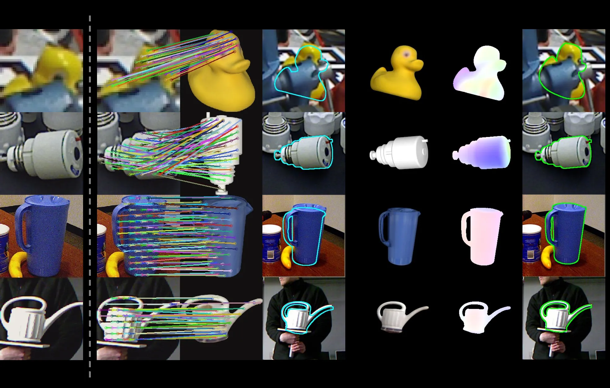
![Figure 6. Qualitative Results of Coarse Estimation. The first two columns on the left display the model's query image and the template with the highest similarity score to the query image. The third and fourth columns compare the CNOS [49] segmentation mask with patches that the model did not classify as 'no-match'. From the fifth to the last columns, the correspondences between the query image and the template, as well as the resulting pose estimation results, are shown.](https://img.032802.xyz/paper-reading/2025/co-op-correspondence-based-novel-object-pose-estimation_2025_Moon/supp_coarse.webp)