【论文笔记】UNOPose: Unseen Object Pose Estimation with an Unposed RGB-D Reference Image
UNOPose: Unseen Object Pose Estimation with an Unposed RGB-D Reference Image
| 方法 | 类型 | 训练输入 | 推理输入 | 输出 | pipeline |
|---|---|---|---|---|---|
| UNOPose | 任意级 | RGBDs | RGBDs | 相对\(\mathbf{R}, \mathbf{t}\) |
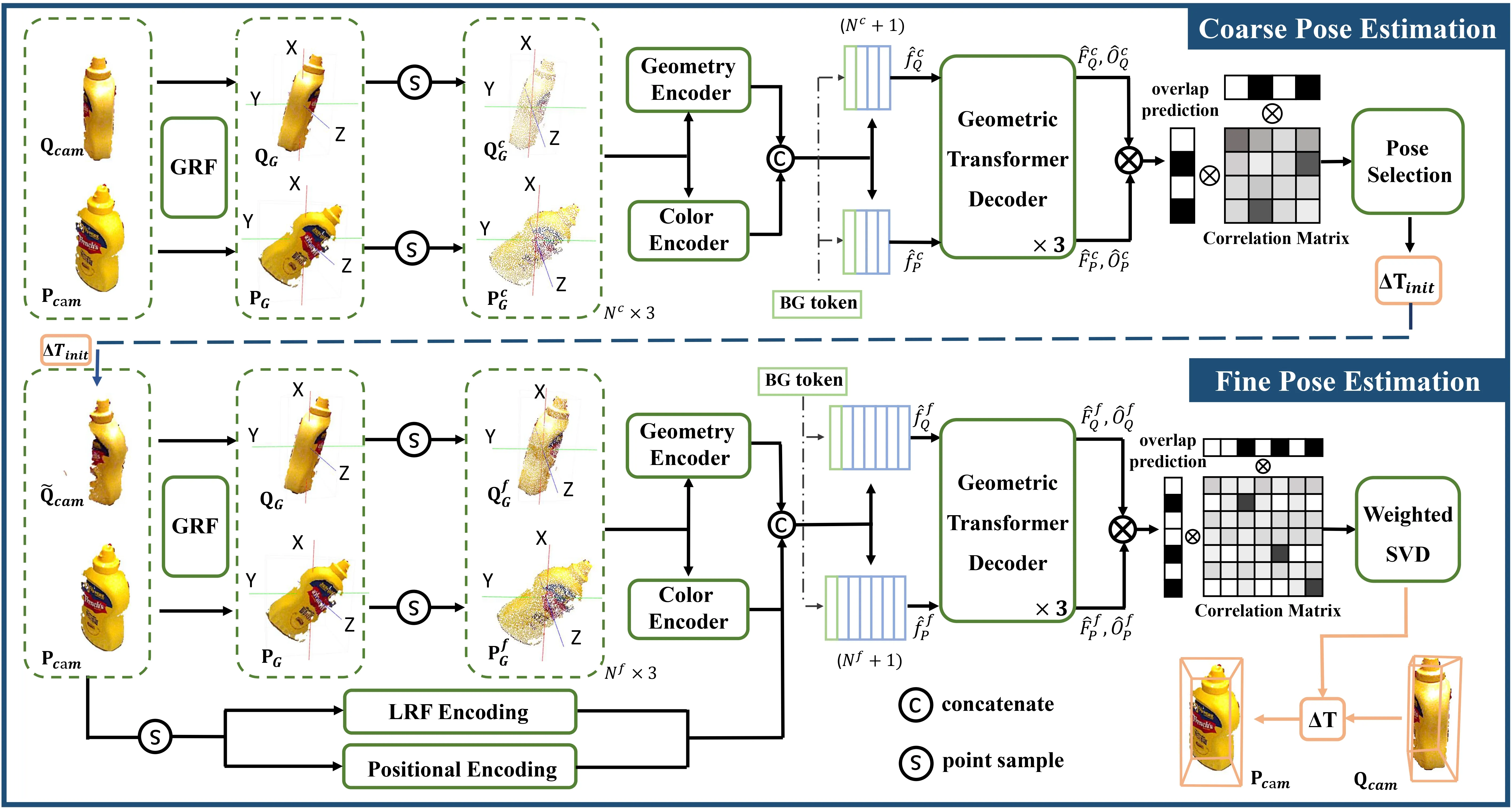
- 2025.05.21:两阶段方法,估计两RGBD图像之间的相对位姿。粗略阶段使用GeoTransformer和DINOv2分别提取点云特征和RGB特征,特征拼接后计算相关矩阵,根据矩阵得到若干匹配点对,从这些匹配点对中选择三个可生成一个刚体变换,即位姿假设,使用距离的倒数进行评分,将评分最高的设置为初始位姿;精细阶段在粗略阶段的基础上增加了局部点云信息和位置编码信息,同样得到相关矩阵后使用加权SVD计算位姿。
Abstract
1. Introduction
![Figure 1. Illustration of unseen object pose estimation. Given a query image presenting a target object unseen during training, we aim to estimate its segmentation and 6DoF pose w.r.t. a reference frame. While previous methods [43, 57, 77, 90] often rely on the CAD model or multiple RGB(-D) images for reference, we merely use one unposed RGB-D reference image.](https://img.032802.xyz/paper-reading/2024/unopose-unseen-object-pose-estimation-with-an-unposed-rgb-d-reference-image_2025_Liu/teaser.webp)
Our contributions can be summarized as follows:
- To the best of our knowledge, we are the first to conduct unseen object 6DoF pose estimation leveraging a single unposed RGB-D reference.
- Based on the BOP Challenge, we devise a new extensive benchmark tailored for unseen object segmentation and pose estimation with one reference. Additionally, we evaluate several traditional and learning-based methods on this benchmark for completeness.
- We introduce UNOPose, a network for learning relative transformation between reference and query objects. To achieve this, we propose the \(SE(3)\)-invariant global and local reference frames, enabling standardized object representations despite variations in pose and size. Furthermore, the network can automatically adjust the confidence of each correspondence by incorporating an overlap predictor.
2. Related Work
3. UNO Object Segmentation and Pose Estimation
3.1. Problem Formulation
假设查询图像中存在一个任意的、未见过的刚性物体,我们的目标是利用一张展示目标物体且无严重遮挡或截断的带掩码RGBD参考图像,估计该物体的掩码\(M_q\)及其6D相对位姿\(\Delta \mathbf{T} \in SE(3)\)。如图1所示,输入包括:
- \([I_q | D_q] \in \mathbb{R}^{H \times W \times 4}\):查询RGBD图像;
- \([I_p | D_p] \in \mathbb{R}^{H \times W \times 4}\) 和 \(M_p \in \mathbb{R}^{H \times W}\):参考RGBD图像及指示目标物体的对应二值掩码;
- \(K_q \in \mathbb{R}^{3 \times 3}\) 和 \(K_p \in \mathbb{R}^{3 \times 3}\):查询图像与参考图像的相机内参。
可选地,如果参考物体在相机坐标系中的位姿\(\mathbf{T}_p \in SE(3)\)已知,则查询物体的位姿\(\mathbf{T}_q \in SE(3)\)可通过\(\mathbf{T}_q = \Delta \mathbf{T} \mathbf{T}_p\)恢复。需要注意的是,从实用性角度出发,该方法不应依赖参考物体的绝对位姿,因为世界坐标系在不同应用中可能任意变化。我们仅在推理阶段对标准物体位姿数据集进行评估时使用参考物体的位姿。
3.2. UNO Object Segmentation
首先,我们需要从杂乱的背景中分割出查询图像中的目标物体。得益于视觉基础模型强大的泛化能力,像“ZeroPose: CAD-Prompted Zero-shot Object 6D Pose Estimation in Cluttered Scenes”、“SAM-6D: Segment Anything Model Meets Zero-Shot 6D Object Pose Estimation”和“CNOS: A Strong Baseline for CAD-based Novel Object Segmentation”等方法能够利用CAD模型对新物体进行有效分割。然而,与以往从多个渲染视图生成多样描述符的方法不同,我们仅能获取单张参考图像。为应对这一挑战,我们采用SAM模型[40]从查询图像中预测所有可能的掩码提议,然后通过余弦相似度比较查询图像与参考图像的DINOv2[65]描述符,对每个掩码提议进行评分,从而筛选出最相似的掩码\(M_q\)。关于UNO分割的更多细节请参见附录。
3.3. UNO Object Pose Estimation
3.3.1. Overview of UNOPose
给定查询图像的预测掩码\(M_q\)和参考图像的掩码\(M_p\),我们从深度图\(D_q\)和\(D_p\)中裁剪出目标物体,并将其反投影到相机空间,得到两个点集\(\mathbf{Q}_{cam} \in \mathbb{R}^{N^Q \times 3}\)和\(\mathbf{P}_{cam} \in \mathbb{R}^{N^P \times 3}\),其中\(N^Q\)和\(N^P\)分别表示查询点云和参考点云的点数。我们的目标是通过最小化对应点距离来恢复相对变换\(\Delta \mathbf{T} = \{\Delta \mathbf{R}, \Delta \mathbf{t}\}\)
\[ \begin{equation}\label{eq1} \min\sum_{(\mathbf{q}, \mathbf{p}) \in \mathbf{C}} \Vert\Delta\mathbf{R}\mathbf{q} + \Delta\mathbf{t} - \mathbf{p}\Vert_2, \end{equation} \]
其中\(\mathbf{C}\)是预测的\(\mathbf{Q}_{cam}\)与\(\mathbf{P}_{cam}\)之间的对应点集。我们利用颜色和几何线索构建该对应关系,并遵循点云配准中广泛使用的由粗到细范式来求解公式\(\eqref{eq1}\)。网络结构如图2所示。
3.3.2. Coarse-to-fine Pose Estimation
Constructing a Pose-invariant Reference Frame.:仅给定一张未标定位姿的参考图像时,待预测的相对位姿在\(SE(3)\)空间中具有任意性,这对实现鲁棒的对应关系构成了重大挑战。因此,我们引入一个位姿无关全局参考框架(GRF),并将\(\mathbf{Q}_{cam}\)和\(\mathbf{P}_{cam}\)转换到GRF中,得到\(\mathbf{Q}_G\)和\(\mathbf{P}_G\)。
具体来说,以\(\mathbf{Q}_{cam}\)为例,将点云转换为全局参考框架(GRF)涉及7D坐标变换\(\{\mathbf{R}_G \in SO(3), \mathbf{t}_G \in \mathbb{R}^3, s_G \in \mathbb{R}\}\):
\[ \begin{equation}\label{eq2} \mathbf{Q}_G = \{\frac{\mathbf{R}_G^T(\mathbf{q} - \mathbf{t}_G)}{s_G} \mid \mathbf{q} \in \mathbf{Q}_{cam}\}. \end{equation} \]
为实现平移不变性,GRF的原点位于物体中心\(\mathbf{c}_Q\);为实现尺寸不变性,点云半径会重新缩放为\(1\),计算方式为:
\[ \begin{equation}\label{eq3} \mathbf{t}_G = \mathbf{c}_Q, \quad s_G = \max_{\mathbf{q} \in \mathbf{Q}_{cam}} \Vert\mathbf{q} - \mathbf{c}_Q\Vert_2. \end{equation} \]
关键在于设计旋转矩阵\(\mathbf{R}_G = [\mathbf{r}_{Gx} | \mathbf{r}_{Gy} | \mathbf{r}_{Gz}]\),其中\(\mathbf{r}_{Gx}, \mathbf{r}_{Gy}, \mathbf{r}_{Gz}\)为\(\mathbf{R}_G\)的三列,用于确保变换后点云的方向不变性。受前人工作“Recognizing Objects in Range Data Using Regional Point Descriptors”、“Structural indexing: efficient 3-D object recognition”和“TOLDI: An effective and robust approach for 3D local shape description”的启发,我们将物体中心的法向量\(\mathbf{n}(\mathbf{c}_Q)\)作为\(\mathbf{r}_{Gz}\),将\(\mathbf{Q}_{cam}\)中所有点投影到\(\mathbf{c}_Q\)的切平面上,通过统计投影向量确定\(\mathbf{r}_{Gx}\),然后通过叉乘\(\mathbf{r}_{Gy} = \mathbf{r}_{Gx} \times \mathbf{r}_{Gz}\)得到\(\mathbf{r}_{Gy}\)。这确保XY平面均匀分割点云,且x轴代表主投影方向。GRF具有\(SE(3)\)无关性,因其可由点云的空间分布唯一确定,使变换后的点云对位姿和尺寸变化具有鲁棒性。
具体来说,我们对协方差矩阵\(\text{Cov}(\mathbf{Q}_{cam}) = \frac{1}{N_Q} \mathbf{Q}_{cam}^T \mathbf{Q}_{cam} - \mathbf{c}_Q \mathbf{c}_Q^T\)进行奇异值分解(SVD),并使用与最小奇异值对应的奇异向量来确定\(\mathbf{r}_{Gz}\):
\[ \begin{equation}\label{eq4} \mathbf{r}_{Gz} = \begin{cases} \mathbf{n}(\mathbf{c}_Q), & \text{if } \mathbf{n}(\mathbf{c}_Q)^T\sum_{\mathbf{q} \in \mathbf{Q}_{cam}}(\mathbf{c}_Q - \mathbf{q}) > 0 \\ -\mathbf{n}(\mathbf{c}_Q), & \text{otherwise} \end{cases} \end{equation} \]
随后,\(r_{Gx}\)的计算公式为:
\[ \begin{equation}\label{eq5} \mathbf{r}_{Gx} = \sum_{\mathbf{q} \in \mathbf{Q}_{cam}}w_q((\mathbf{q} - \mathbf{c}_Q) - \mathbf{r}_{Gz}^T(\mathbf{q} - \mathbf{c}_Q)\mathbf{r}_{Gz}), \end{equation} \]
其中\(w_q\)是关于点\(\mathbf{q}\)与物体中心\(\mathbf{c}_Q\)之间距离的权重(具体细节见附录)。
以往的工作“Leveraging SE(3) Equivariance for Self-Supervised Category-Level Object Pose Estimation”、“CPPF: Towards Robust Category-Level 9D Pose Estimation in the Wild”和“Rotation-Invariant Transformer for Point Cloud Matching”通常依赖复杂网络或计算成本高昂的PPF特征来实现\(SE(3)\)无关性。相比之下,我们的变换方法计算效率高,并且能够无缝适配多种网络架构。
Coarse Pose Estimation.:给定GRF中的点云\(\mathbf{Q}_G\)和\(\mathbf{P}_G\),我们采样两个稀疏点集\(\mathbf{Q}_G^c \in \mathbb{R}^{N^c \times 3}\)和\(\mathbf{P}_G^c \in \mathbb{R}^{N^c \times 3}\)以高效获取粗位姿初始化\(\Delta \mathbf{T}_{init}\)。具体而言,我们利用几何编码器“GeoTransformer: Fast and Robust Point Cloud Registration with Geometric Transformer”和颜色编码器“DINOv2: Learning Robust Visual Features without Supervision”分别提取点云和RGB特征。特征进一步拼接为\(f_Q^c \in \mathbb{R}^{N^c \times d}\)和\(f_P^c \in \mathbb{R}^{N^c \times d}\),其中\(d\)为嵌入维度。遵循“SAM-6D: Segment Anything Model Meets Zero-Shot 6D Object Pose Estimation”,我们添加可学习的背景标记以分配非重叠点。这些嵌入表示为\(\hat{f}_Q^c \in \mathbb{R}^{(N^c + 1) \times d}\)和\(\hat{f}_P^c \in \mathbb{R}^{(N^c + 1) \times d}\),并通过三个堆叠的Geometric Transformer解码模块进行处理。
最后一个解码器的输出\(\hat{F}_Q^c \in \mathbb{R}^{(N^c + 1) \times D}\)和\(\hat{F}_P^c \in \mathbb{R}^{(N^c + 1) \times D}\)是用于构建相关矩阵的逐点特征。然而,在我们的场景中,重叠率可能受到视点、遮挡或深度噪声等复杂因素的影响。为解决这一问题,网络额外预测重叠置信度\(\hat{O}_Q^c \in \mathbb{R}^{(N^c + 1) \times 1}\)和\(\hat{O}_P^c \in \mathbb{R}^{(N^c + 1) \times 1}\),表示各点属于重叠区域的概率。因此,重叠感知相关矩阵\(\mathbf{X}_c \in \mathbb{R}^{(N^c + 1) \times (N^c + 1)}\)可通过下式计算:
\[ \begin{equation}\label{eq6} \mathbf{X}^c = \text{softmax}[(\hat{O}_Q^c \odot \hat{F}_Q^c)(\hat{O}_P^c \odot \hat{F}_P^c)^T]. \end{equation} \]
这里\(\odot\)表示元素级乘法。\(\mathbf{X}^c\)中的每个元素表示\(\mathbf{Q}^c\)与\(\mathbf{P}^c\)中点对之间的相关分数。
在计算出相关矩阵\(\mathbf{X}^c\)后,我们可以提取\(\mathbf{Q}^c\)和\(\mathbf{P}^c\)之间所有可能的对应点对及其相关分数,从而求解公式\(\eqref{eq1}\)。具体来说,我们首先根据\(\mathbf{X}^c\)的分布采样\(N_H\)个点对三元组,生成位姿假设。然后,每个位姿假设\(\Delta \mathbf{T}_h = \{\Delta \mathbf{R}_h, \Delta \mathbf{t}_h\}\)按照“SurfEmb: Dense and Continuous Correspondence Distributions for Object Pose Estimation with Learnt Surface Embeddings”和“SAM-6D: Segment Anything Model Meets Zero-Shot 6D Object Pose Estimation”中的方法,通过距离\(D_h\)的倒数进行评分:
\[ \begin{equation}\label{eq7} \begin{aligned} D_h &= \frac{1}{N^c}\sum_{\mathbf{p}^c \in \mathbf{P}^c}\min_{\mathbf{q}^c \in \mathbf{Q}^c}\Vert\Delta\mathbf{R}_h^T(\mathbf{q}^c - \Delta\mathbf{t}_h) - \mathbf{p}^c\Vert_2, \\ \xi_h &= \frac{1}{D_h}, \quad h = 1, 2, \cdots, N_H. \end{aligned} \end{equation} \]
得分\(\xi_h\)最高的位姿假设被选为初始位姿预测值\(\Delta \mathbf{T}_{init} = \{\Delta \mathbf{R}_{init}, \Delta \mathbf{t}_{init}\}\),并进一步用于变换下一阶段的输入。
Fine Pose Estimation.:在使用初始位姿预测\(\Delta \mathbf{T}_{init}\)将\(\mathbf{Q}_{cam}\)变换为\(\tilde{\mathbf{Q}}_{cam}\)之后,我们在两个密集点集,即\(\tilde{\mathbf{Q}}^f \in \mathbb{R}^{N^f \times 3}\)和\(\mathbf{P}^f \in \mathbb{R}^{N^f \times 3}\)之间执行精细匹配过程,以获得更精确的位姿。该网络通过分层编码范式利用几何细节,包括位置编码层和局部参考框架编码层。对于每个点,我们首先使用小型PointNet,即“PointNet: Deep Learning on Point Sets for 3D Classification and Segmentation”对其全局位置进行编码,然后构建\(SE(3)\)无关局部参考框架(LRF)以收集局部描述符。这两种编码相互补充,因为局部描述符捕获小邻域内的精细几何结构,而位置编码层提供全局几何上下文。
以\(\tilde{\mathbf{Q}}^f\)为例,构建局部参考框架(LRF)编码的过程如下:对于\(\tilde{\mathbf{Q}}^f\)中的每个点\(\tilde{\mathbf{q}}^m\),通过将\(\tilde{\mathbf{q}}^m\)的\(N_D\)个邻近点分组,构建局部区域集合\(\tilde{\mathcal{Q}}^m = \{\tilde{\mathbf{q}}_j, \text{where } \Vert\tilde{\mathbf{q}}_j - \tilde{\mathbf{q}}^m\Vert_2 \leq r\}_{j = 1}^{N_D}\)。LRF的变换位姿\(\{\mathbf{R}_L^m, \mathbf{t}_L^m, s_L^m\}\)的计算方式与GRF类似(见公式\(\eqref{eq3}\)、\(\eqref{eq4}\)、\(\eqref{eq5}\)),区别在于LRF基于局部点集构建,而GRF基于整个点云。通过计算变换位姿,我们将局部点描述符计算为:
\[ \begin{equation}\label{eq8} \begin{aligned} \mathcal{Q}_L^m &= \tilde{\mathcal{Q}}_L^m = \{(\mathbf{R}_L^m)^T(\frac{\tilde{\mathbf{q}}_j - \mathbf{t}_L^m}{s_L^m})\}_{j = 1}^{N_D}, \\ \mathbf{Q}_L^f &= \{\mathcal{Q}_L^m\}_{m = 1}^{N^f}. \end{aligned} \end{equation} \]
类似地,我们将\(\mathbf{P}^f\)变换为\(\mathbf{P}_L^f\)。注意,由于LRF是位姿无关的,因此\(\mathcal{Q}_L^m = \tilde{\mathcal{Q}}_L^m\)。然后,通过三层MLP从\(\mathbf{Q}_L^f\)和\(\mathbf{P}_L^f\)中提取LRF编码。
位置编码和LRF编码与几何和颜色特征相结合,作为几何Transformer的输入。与初始位姿预测类似,通过解码这些特征,我们获得精细的逐点特征\(\hat{F}^f_Q\)、\(\hat{F}^f_P\)以及重叠置信度\(\hat{O}^f_Q\)、\(\hat{O}^f_P\),然后利用这些结果得到考虑重叠区域的精细相关矩阵\(\mathbf{X}^f \in \mathbb{R}^{(N^f + 1) \times (N^f + 1)}\)。最终位姿\(\Delta \mathbf{T}\)通过使用加权SVD算法对\(\mathbf{X}^f\)求解公式\(\eqref{eq1}\)来预测。