【论文笔记】MRC-Net: 6-DoF Pose Estimation with MultiScale Residual Correlation

MRC-Net: 6-DoF Pose Estimation with MultiScale Residual Correlation

方法	类型	训练输入	推理输入	输出	pipeline
MRC-Net	（貌似是）实例级	RGB + 物体类别	RGB + 物体类别	绝对\(\mathbf{R}, \mathbf{t}\)

• 2025.02.22：说实话这篇文章没怎么看懂，感觉正文和图片对不上...，但是里面有旋转图片的数据增强操作，可以学一下

Abstract

1. Introduction

Figure 1. MRC-Net features a single-shot sequential Siamese structure of two stages, where the second stage conditions on the first classification stage outcome through multi-scale residual correlation of poses between input and rendered images.

To summarize, the main contributions of this work are:

• MRC-Net, a novel single-shot approach to directly estimate the 6-DoF pose of objects with known 3D models from monocular RGB images. Unlike prior methods, our approach performs classification and regression sequentially, guiding residual pose regression by conditioning on classification outputs. Moreover, we introduce a custom classification design based on soft labels, to mitigate symmetry-induced ambiguities.
• A novel MRC layer that implicitly captures correspondences between input and rendered images at both global and local scales. Since MRC-Net is end-to-end trainable, this encourages the correlation features to be more discriminative, and avoids the need for complicated post-processing procedures.
• State-of-the-art accuracy on a variety of BOP benchmark datasets, advancing average recall by 2.4% on average compared to results reported by competing methods.

2. Related Work

3. Methodology

Figure 2. MRC-Net Architecture. The classifier and regressor stages employ a Siamese structure with shared weights. Both stages take the object crop and its bounding box map as input, and extract image features to detect the visible object mask, which are concatenated together to estimate object pose. The classifier first predicts pose labels. These predictions, along with the 3D CAD model, are then used to render an image estimate, which serves as input for the second stage. Features from the rendered image are correlated with those from real images in the MRC layer. These correlation features undergo ASPP processing within the rendered branch to regress the pose residuals.

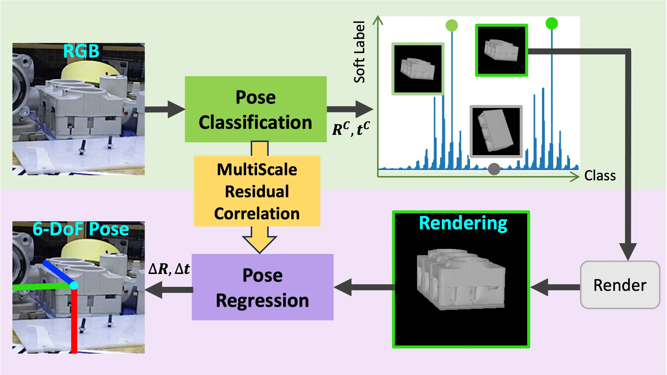
• 给定crop后的RGB图和物体的CAD模型，MRC-Net估计物体的\(\mathbf{R}\)和\(\mathbf{t}\)，如图2所示；

• 分类阶段和残差回归阶段共同解决三个共存的问题：

  • 3D旋转\(\mathbf{R} \in SO(3)\)；
  • 2D平面内平移\((t_x, t_y) \in \mathbb{R}^2\)；
  • 1D深度\(t_z \in \mathbb{R}\)；

1. 在第一个阶段：

   1. 方法使用一个位姿分类器处理RGB图，得到位姿标签\(\mathbf{R}_c\)和\((t_x^c, t_y^c, t_z^c)\)；
   2. 使用预测出的位姿标签，结合物体的CAD，渲染出物体的一幅图片；
   3. 为了量化旋转\(SO(3)\)，方法根据“Generating Uniform Incremental Grids on SO(3) Using the Hopf Fibration”，生成了旋转原型集合\(\{\mathbf{R}_k\}_{k=1}^K\)，这可以将旋转空间分为\(K\)个bucket；
   4. 同样对于\(t_x\)，\(t_y\)和\(t_z\)，方法根据“CDPN: Coordinates-Based Disentangled Pose Network for Real-Time RGB-Based 6-DoF Object Pose Estimation”的SITE，将平移转换表示为\((\tau_x, \tau_y, \tau_z)\)，然后分别生成2D和1D的空间均匀网格；

2. 在第二个阶段：

   1. 将第一个阶段渲染后的物体图像和它的bounding box输入，基于“渲染-比较”，估计输入图像和渲染图像之间的残差位姿\(\Delta \mathbf{R}\)和\((\Delta \tau_x, \Delta \tau_y, \Delta \tau_z)\)；
   2. 这样，第二阶段的位姿估计就受到了第一阶段位姿分类的指导，简化了回归任务；
   3. 这里会使用MRC模块计算输入图像和渲染图像之间之间的相关性；

3. 最后，两个阶段的预测结果会进行结合，得到最终的6-DoF位姿，即：\(\hat{\mathbf{R}} = \Delta \mathbf{R} \mathbf{R}^c\)和\(\hat{\tau}_i = \tau_i^c + \Delta \tau_i, i \in \{x, y, z\}\)。

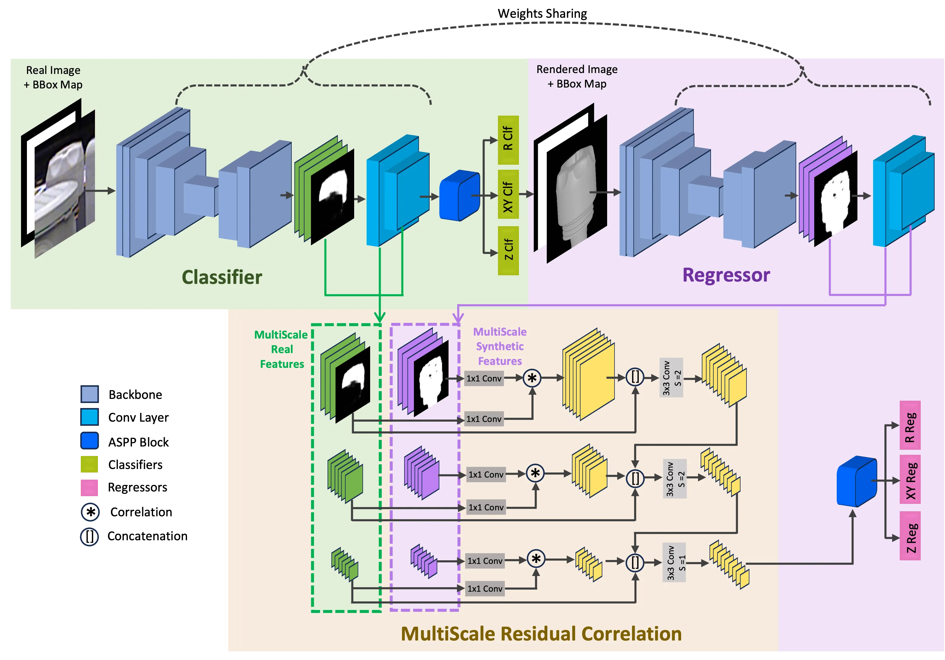
3.1. MultiScale Residual Correlation

Figure 3. Comparison of (a) conventional approaches and (b) our proposed approach leveraging feature correlations to estimate residual pose. Instead of predicting an intermediate flow field, we directly feed multi-scale feature correlations into the regression head in an end-to-end fashion. These features are discriminative and eliminate the need for post refinement, outlier removal or multiview renderings.

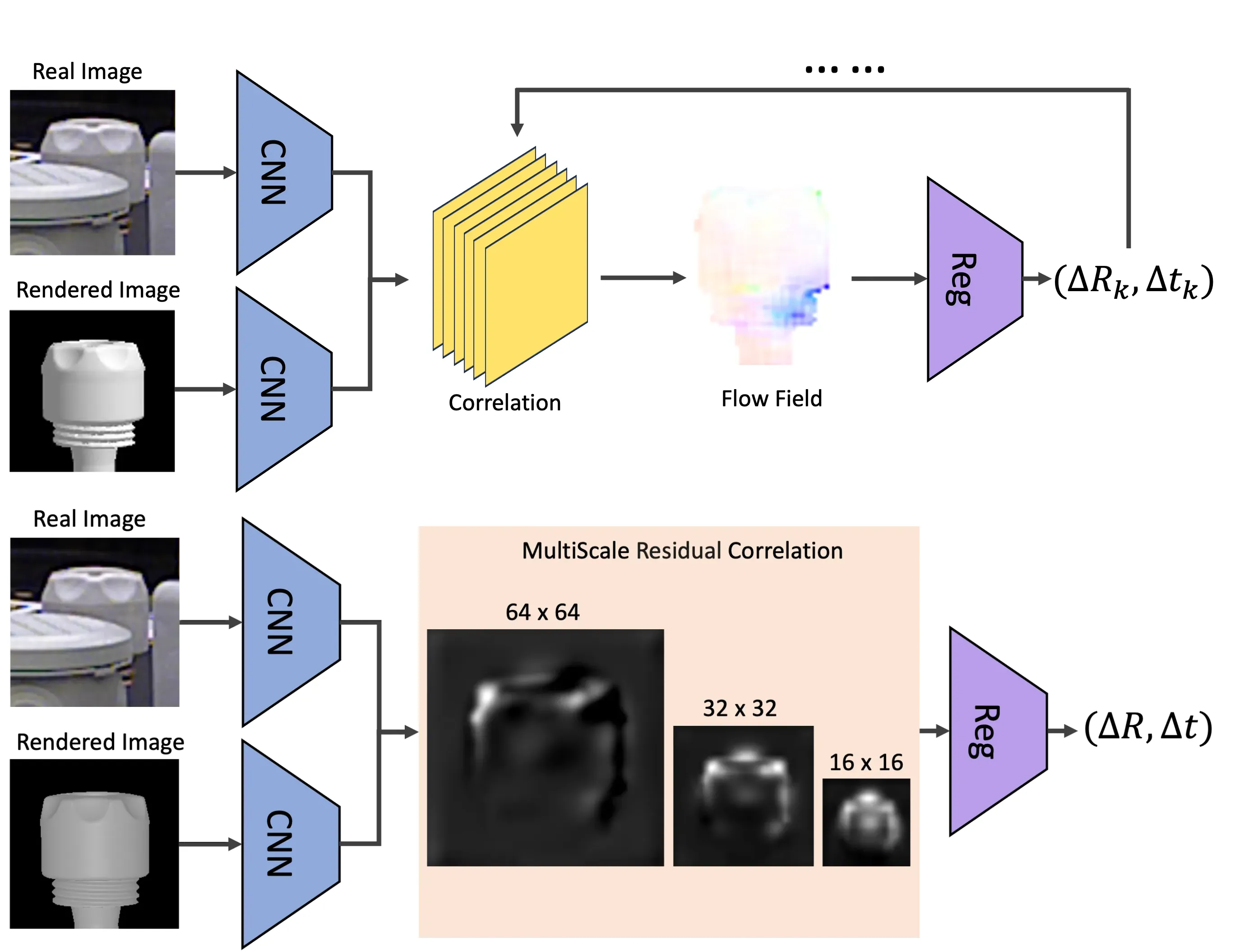
MRC在三个比例下计算真实图像和渲染图像特征体之间的相关性。随后，相关特征会被送入回归头中，产生残差位姿。

在计算相关性时，方法遵循“PWC-Net: CNNs for Optical Flow Using Pyramid, Warping, and Cost Volume”，将相关性限制在\(P \times P\)的窗口中。数学上，给定维度均为\(d \times H \times W\)的真实图像特征体\(\mathbf{f}_r\)和渲染图像特征体\(\mathbf{f}_s\)，得到维度为\(P^2 \times H \times W\)的相关体\(\mathbf{c}\)，计算如下：

\[ \mathbf{c}(\mathbf{v}, \mathbf{x}) = \frac{1}{\sqrt{d}} \mathbf{f}_s(\mathbf{x})^T \mathbf{f}_r(\mathbf{x} + \mathbf{v}), \quad \forall \mathbf{v}: \Vert \mathbf{v} \Vert_\infty \leq P, \]

其中，\(\mathbf{x}\)是每个像素位置，\(\mathbf{v}\)是偏移量，\(\Vert \cdot \Vert_\infty\)是无穷范数，即向量中每个元素绝对值的最大值。

3.2. Technical Details

Soft labels for classification

方法将位姿估计视作分类问题，那么首先需要定义位姿的类别，而将物体旋转分配给离散的位姿bucket是一项复杂的挑战。

具体来说，物体旋转可能位于\(SO(3)\) bucket的边界上，对于多个旋转原型有相同的测地距离，导致了固有的歧义。此外，某些物体存在对称性，使得同一RGB图会对应多个刚体变换。为了解决这个问题，方法在分类中使用软标签，根据位姿误差指标，对物体是否属于某个view bucket进行二进制概率建模。“EPro-PnP: Generalized End-to-End Probabilistic Perspective-n-Points for Monocular Object Pose Estimation”中探讨了类似的概念，其中物体位姿的连续分布是根据重投影误差定义的。相比之下，方法为旋转类制定软赋值，为问题提供了一个新颖的视角。

具体来说，给定带注释的物体位姿\((\mathbf{R}^*, \mathbf{t}^*)\)，方法将旋转标签定义为：

\[ l_k^\mathbf{R} = \exp\left\{-\frac{\rho_\text{pose_symm}(\mathbf{R}^*, \mathbf{t}^*; \mathbf{R}_k, \mathbf{t}^*)}{\sigma}\right\}, \]

其中，\(k = 1, \cdots, K\)，\(\rho_\text{pose_symm}(\mathbf{R}^*, \mathbf{t}^*; \mathbf{R}_k, \mathbf{t}^*)\)测量物体位姿\((\mathbf{R}_1, \mathbf{t}_1; \mathbf{R}_k, \mathbf{t}_k)\)之间的对称感知距离，\(\sigma > 0\)是调节分类标签集中度的超参数。

本质上来说，软标签描述了以带注释旋转\(\mathbf{R}^*\)为中心的旋转\(\mathbf{R}_k\)的指数加权组合，权重由它们的对称感知距离决定。

相似的，为了用于生成平移的软标签，方法将\((\tau_x, \tau_y)\)均匀量化为\(64 \times 64\)的网格，将\(\tau_z\)量化为指定范围内的\(1000\)个区间。最后，使用以真值位置为中心的高斯函数计算平移标签。

Loss functions

旋转分类任务是通过最小化焦点损失\(\mathcal{L}_\text{cls}^\mathbf{R}\)来训练的，定义为：

\[ \mathcal{L}_\text{cls}^\mathbf{R} = \sum_{k = 1}^{K} - w^+ l_{k}^\mathbf{R} (1 - \hat{p}_k)^2 \log \hat{p}_k - (1 - l_{k}^\mathbf{R}) \hat{p}_k^2 \log (1 - \hat{p}_k), \]

其中，\(\{\hat{p}_k\}_{k = 1}^K\)是分类器预测的概率。

注意，方法使用成对二进制编码以允许同时存在多个类隶属关系，并引入一个加权参数\(w^+ > 0\)，在这里为100，以解决类不平衡问题。

为了求解平移，\(xy\)和\(z\)分类任务都对多焦点损失进行了优化：

\[ \mathcal{L}_\text{cls}^i = -\left(1 - \sum_{j = 1}^{n_i} l_j^i \hat{p}_j^i \right)^2 \log \left(\sum_{j = 1}^{n_i} l_j^i \hat{p}_j^i\right), \quad i \in \{xy, z\}, \]

其中，\(l_j^{xy}\)和\(l_j^z\)是\(xy\)和\(z\)的平移软标签，\(\hat{p}_j^{xy}\)和\(\hat{p}_j^z\)是预测概率，\(n_{xy} = 64\)和\(n_z = 1000\)。在推理时，方法为所有三个任务选择置信度最高的类。

旋转回归任务预测渲染物体和真实物体之间的残差旋转\(\Delta \mathbf{R}\)。这个量通常在较小的位姿角度下具有局部性，并且更容易通过回归进行学习。将来自分类器的粗略旋转\(\mathbf{R}_c\)和\(\Delta \mathbf{R}\)结合，就能够得到细粒度旋转预测\(\hat{\mathbf{R}} = \Delta \mathbf{R} \mathbf{R}_c\)。方法使用“On the Continuity of Rotation Representations in Neural Networks”中的旋转表示。

同样的，方法将两个阶段的平移进行结合，来得到最终的物体平移：\(\hat{\tau}_i = \tau_i^c + \Delta \tau_i, i \in \{x, y, z\}\)。

为了训练旋转回归任务，方法采用的解耦损失函数：

\[ \mathcal{L}_\text{reg}^\mathbf{R} = \rho_\text{pose_sym}(\Delta \mathbf{R} \mathbf{R}^{c}, \mathbf{t}^*; \mathbf{R}^*, \mathbf{t}^*), \]

其中，\((\mathbf{R}^*, \mathbf{t}^*)\)是带注释的物体位姿。

其余两项\(\mathcal{L}_\text{reg}^{xy}\)和\(\mathcal{L}_\text{reg}^z\)的定义类似。

最终的损失函数是通过各个项的加权组合形成的：

\[ \mathcal{L} = w_\text{cls}^\mathbf{R} \mathcal{L}_\text{cls}^\mathbf{R} + w_\text{cls}^{xy} \mathcal{L}_\text{cls}^{xy} + w_\text{cls}^z \mathcal{L}_\text{cls}^z + w_\text{reg}^\mathbf{R} \mathcal{L}_\text{reg}^\mathbf{R} + w_\text{reg}^{xy} \mathcal{L}_\text{reg}^{xy} + w_\text{reg}^z \mathcal{L}_\text{reg}^z + w^M \mathcal{L}^M, \]

其中，\(\mathcal{L}^M\)是可见掩码项，定义为二元交叉熵损失，且\(w^M > 0\)是其权重。

Perspective correction

由于方法是在以感兴趣对象为中心的裁剪视图上进行操作的，它可能缺乏全局上下文信息。

具体而言，正如“CLIFF: Carrying Location Information in Full Frames into Human Pose and Shape Estimation”中所强调的，可能会出现这样的情况：网络被迫对外观相同的图像裁剪预测出不同的姿态，从而在监督过程中造成混淆。

缓解这一挑战的一个常见策略是将以自我为中心的旋转转换为以环境为中心的旋转。然而，这种解决方案需要对物体中心进行准确预测，并且没有考虑到平移因素。相反，我们采用了与“CLIFF: Carrying Location Information in Full Frames into Human Pose and Shape Estimation”类似的方法，额外将边界框特征的全局信息纳入到每个分类器中。

我们输入\(\left[\frac{b_x - c_x}{f}, \frac{b_y - c_y}{f}, \frac{s_{bbox}}{f}\right]\)，其中\(b_x\)和\(b_y\)是边界框的中心，\(c_x\)和\(c_y\)是相机主点，\(f\)是焦距。

在我们的实验中，按照惯例，我们直接从数据集注释中获取相机的焦距和主点。与“CLIFF: Carrying Location Information in Full Frames into Human Pose and Shape Estimation”不同的是，我们在分类阶段之后得到粗略的平移估计值\((t_{cx}, t_{cy}, t_{cz})\)。随后，在回归阶段的“渲染-比较”中，方法直接将\(\left(\frac{t_{cx}}{t_{cz}}, \frac{t_{cy}}{t_{cz}}, s_{bbox}^f\right)\)输入到回归头中，而不是输入边界框中心。这一修改确保了回归器能够获知真实的投影物体中心，从而有助于准确预测残差。

4. Experiments

4.1. Setup

4.2. Ablation Studies

(a) Comparison of hard and soft labels. The table illustrates performance when trained with and without soft labels.

Method	ARVSD↑	ARMSSD↑	ARMSPD↑	AR↑
Hard Label	67.8	72.2	84.6	74.8
Soft Label	70.6	74.7	86.0	77.1

(b) Comparison of parallel and sequential designs. ClfOnly denotes a classification-only model. MultiTask is a parallel baseline architecture. FeatConcat sends concatenated real and rendered image features to the regressor. SSCorr use single-scale feature correlation, while MRC-Net uses multi-scale feature correlation. P denotes parallel classification and regression, while S denotes sequential.

Type	Method	ARVSD↑	ARMSSD↑	ARMSPD↑	AR↑
-	ClfOnly	55.6	62.8	77.4	65.3
P	MultiTask	55.3	62.7	76.6	64.9
S	FeatConcat	69.4	73.5	85.7	76.2
S	SSCorr	69.8	73.9	85.8	76.5
S	MRC-Net	70.6	74.7	86.0	77.1

(c) Impact of perspective correction (PerspCrrct) and test-time augmentation (TTA). Dropping perspective correction results in noticeable degradation in performance, while omitting TTA has a more modest impact.

Table 1. Ablation studies of our method on T-LESS dataset [16].

Method	ARVSD↑	ARMSSD↑	ARMSPD↑	AR↑
w/o PerspCrrct	69.9	74.1	85.9	76.6
w/o TTA	70.4	74.1	85.7	76.7
Full model	70.6	74.7	86.0	77.1

4.3. Comparison with State-of-the Art

(a)

Method	T-LESS	ITODD	YCB-V	LM-O	Avg.
EPOS [17]	46.7	18.6	49.9	54.7	42.5
CDPNv2 [29]	40.7	10.2	39.0	62.4	38.1
DPODv2 [44]	63.6	-	-	58.4	-
PVNet [40]	-	-	-	57.5	-
CosyPose [26]	64.0	21.6	57.4	63.3	51.6
SurfEmb [13]	74.1	38.7	65.3	65.6	60.9
SC6D [2]	73.9	30.3	61.0	-	-
SCFlow [11]	-	-	65.1	68.2	-
PFA [22]	-	-	61.5	67.4	-
CIR [33]	-	-	-	65.5	-
SO-Pose [7]	-	-	-	61.3	-
NCF [23]	-	-	67.3	63.2	-
CRT-6D [3]	-	-	-	66.0	-
MRC-Net	77.1	39.3	68.1	68.5	63.3

(b)

Table 2. Comparison with state-of-the-srt RGB methods on the BOP benchmarks. We report Average Recall in % on (a) T-LESS, ITODD, YCB-V, and LM-O datasets trained with purely synthetic images, and (b) T-LESS and YCB-V datasets also trained with real images. We highlight the best results in bold and underline the second best results. "-" denotes results missing from the original paper.

Method	T-LESS	YCB-V	Avg.
CDPNv2 [29]	47.8	53.2	50.5
CosyPose [26]	72.8	82.1	77.4
SurfEmb [13]	77.0	71.8	74.4
SC6D [2]	78.0	78.8	78.4
SCFlow [11]	-	82.6	-
CIR [33]	71.5	82.4	77.0
SO-Pose [7]	-	71.5	-
NCF [23]	-	77.5	-
CRT-6D [3]	-	75.2	-
MRC-Net	79.8	81.7	80.8

Table 3. Comparison on the YCB-V Dataset. We report the ADD(-S), AUC of ADD-S, and AUC of ADD(-S) metrics in %. We highlight the best results in bold and underline the second best results. "-" denotes results missing from the original paper and ^∗ denotes results obtained using the FCOS detector [29].

Method	ADD(-S) ↑	AUC ADD-S ↑	AUC ADD(-S) ↑
SegDriven [19]	39.0	-	-
SingleStage [20]	53.9	-	-
CosyPose [26]	-	89.8	84.5
RePose [24]	62.1	88.5	82.0
GDR-Net [52]	60.1	91.6	84.4
SO-Pose [7]	56.8	90.9	83.9
ZebraPose [47]∗	80.5	90.1	85.3
SCFlow [11]	70.5	-	-
DProST [39]	65.1	-	77.4
CheckerPose [31]∗	81.4	91.3	86.4
MRC-Net	81.2	95.0	92.3
MRC-Net∗	83.6	97.0	94.3

Figure 4. Qualitative comparison of results on T-LESS: (a) Original RGB image, (b) MRC-Net, (c) CosyPose initialized PFA [22], (d) SC6D [2], and (e) ZebraPose [47]. The object’s 3D model is projected with estimated 6D pose and overlaid on original images with distinct colors. Red boxes denote cases where pose predictions are distinctly different across the methods. MRC-Net outperforms the state-of-art models particularly under heavy occlusion. (Best viewed when zoomed in.)

Runtime comparisons. We run CIR [33], PFA [22], SurfEmb [13], GDR-Net [52], SC6D [2] and MRC-Net (Ours) on the same AWS EC2 P3.2Xlarge instance, and report the average runtime in milliseconds to infer one object pose. For methods with ^∗, the time required for pose initialization, typically involving the execution of an additional off-the-shelf network, is not included.

Methods	[33]∗	[22]∗	[13]	[52]	[2]	MRC-Net
Time (ms)	2542	88	1121	26	25	61

5. Conclusions and Limitations