【论文笔记】ES6D: A Computation Efficient and Symmetry-Aware 6D Pose Regression Framework

发表于 2025-04-23 更新于 2025-05-08 分类于读万卷书阅读次数： Waline：本文字数： 4.3k 阅读时长 ≈ 15 分钟

In this paper, a computation efficient regression framework is presented for estimating the 6D pose of rigid objects from a single RGB-D image, which is applicable to handling symmetric objects. This framework is designed in a simple architecture that efficiently extracts point-wise features from RGB-D data using a fully convolutional network, called XYZNet, and directly regresses the 6D pose without any post refinement. In the case of symmetric object, one object has multiple ground-truth poses, and this one-to-many relationship may lead to estimation ambiguity. In order to solve this ambiguity problem, we design a symmetry-invariant pose distance metric, called average (maximum) grouped primitives distance or A(M)GPD. The proposed A(M)GPD loss can make the regression network converge to the correct state, i.e., all minima in the A(M)GPD loss surface are mapped to the correct poses. Extensive experiments on YCB-Video and TLESS datasets demonstrate the proposed framework's substantially superior performance in top accuracy and low computational cost. The relevant code is available in https://github.com/GANWANSHUI/ES6D.git.

ES6D: A Computation Efficient and Symmetry-Aware 6D Pose Regression Framework

方法	类型	训练输入	推理输入	输出	pipeline
ES6D	实例级（该方法针对对称物体设计）	RGBD + CAD	RGBD + CAD	绝对\(\mathbf{R}, \mathbf{t}\)

2025.05.08：这篇文章主要解决的是对称物体的6D位姿估计问题，使用Grouped Primitives (GP)来对物体分类，GP可以将同一类别的物体（类别是GP的类别，而不是物体的类别）抽象为几个点，以避免由形状引起的不确定性；还设计了位姿距离loss A(M)GPD，该loss曲线上的每一个极小值点都可以映射到一个正确的姿态。

Abstract

1. Introduction

Figure 1. Comparison of A(M)GPD and ADD-S. Axis X shows the rotation angle of the object (from 0° to 360°). Axis Y shows the calculated distance. We set the initial pose as the ground truth. As we can see, all minima are mapped to correct poses in the A(M)GPD curve and several minima point to incorrect poses in the ADD-S curve.

\[ \begin{equation}\label{eq1} l = \text{loss}(p, \hat{p}) = \text{loss}(N(I, w), \hat{p}), \end{equation} \]

In summary, the main contributions of this work are as follows.

We propose a novel feature extraction network XYZNet for the RGB-D data, which is suitable for pose estimation with low computational cost and superior performance.
The compact shape representation GP and the distance metric A(M)GPD are introduced to handle symmetries. The loss based on A(M)GPD can constrain the regression network to converge to the correct state.
A numerical simulation and visualization method is carried out to analyze the validity of the A(M)GPD loss. This analytical method is applicable to other frameworks in 6D pose estimation.
The framework ES6D is proposed by using XYZNet and the A(M)GPD loss and achieves competitive performance on the YCB-Video and T-LESS datasets.

3. The Proposed Method

3.1. Overview

Figure 2. Network overview. First, the RGB-XYZ data is generated from the RGB-D image. The RGB-XYZ data is fed into a CNN module to extract local features, which encode color and geometry information. Second, the point cloud features are obtained by a PointNet-like CNN module and padded to the same size as the local features. Then, the local features and point cloud features are concatenated as the point-wise features for poses estimation. Finally, the pose with the maximum confidence is chosen as the final result.

本文的目的是从一幅RGBD图像中检测出刚性物体，并在相机坐标系中估计出相应的旋转\(R \in SO(3)\)和平移\(\boldsymbol{t} \in \mathbb{R}^3\)。为此提出了如下的两阶段方案。

在第一阶段，利用“PoseCNN: A Convolutional Neural Network for 6D Object Pose Estimation in Cluttered Scenes”的分割网络来获取目标物体的掩码和边界框。由边界框裁剪得到的每个掩码以及RGBD图像块都会被传送到第二阶段。

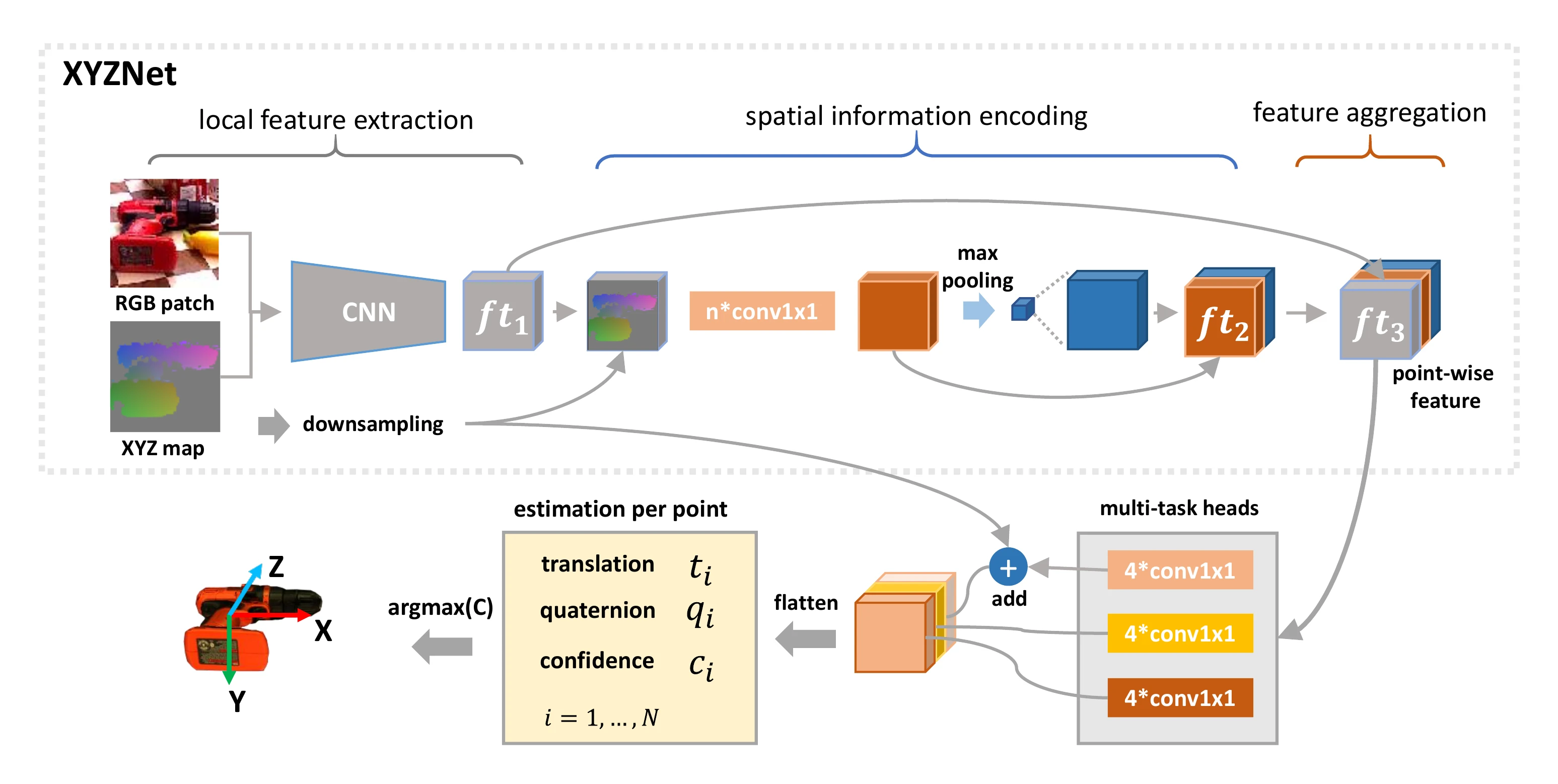
在第二阶段，提出了一个名为ES6D的实时框架来估计物体位姿。该框架的流程如图2所示。首先，经过归一化处理后，带掩码的深度像素会被转换为XYZ map。其次，XYZNet从RGB图像块和XYZ map的拼接结果中提取point-wise特征。然后，利用三个卷积头来预测point-wise平移偏移量、四元数以及置信度。最后，选择置信度最高的位姿作为最终结果。

3.2. Point-wise feature extraction

之前的工作“PVN3D: A Deep Point-wise 3D Keypoints Voting Network for 6DoF Pose Estimation”和“DenseFusion: 6D Object Pose Estimation by Iterative Dense Fusion”已经证明，对于6D位姿估计而言，来自RGBD数据的point-wise特征比来自RGB图像的特征更加有效且稳健。最先进的方法PVN3D采用一种异构结构，该结构通过PointNet++获取点云特征，然后通过索引操作将点云特征与RGB特征链接起来。PointNet++通过一系列集合抽象层（Set Abstraction Layers, SAL）来提取局部特征，这些层会在预定义的搜索半径内对点云进行分组。然而，处理大量的点云非常耗时，并且如果我们减少集合抽象层的数量，其表示能力就会下降。2D卷积操作的一个特点是对相邻信息进行分组以提取局部特征。因此，所提出的XYZNet旨在通过对RGB-XYZ图像执行2D卷积操作来同时提取局部特征。

首先，经过掩码处理的深度像素被转换为点云\(\mathcal{P} = \{(x_i, y_i, z_i)\}_{i = 1}^N\)，然后使用点的中心\(\boldsymbol{p}_c = \text{mean}(\mathcal{P})\)和一个比例因子\(\gamma\)，将点\(P\)进行平移和缩放到\([-1, 1]\)区间。归一化后的点记为\(\dot{\mathcal{P}} = \{(\dot{x}_i, \dot{y}_i, \dot{z}_i)\}_{i = 1}^N\)，并被格式化为一个XYZ map。通过将XYZ map与相应的RGB patch进行拼接，就可以得到严格对齐的RGB-XYZ数据。“A Unified Framework for Multi-View Multi-Class Object Pose Estimation”中的方法也采用了2D卷积网络从XYZ map中提取点云特征，但其性能远不如异构结构的方法（PVN3D和DenseFusion）。造成这种情况的主要原因是，当在XYZ map上使用2D卷积操作时，点云的空间信息会被丢弃。基于上述观察，我们设计了XYZNet，如图2所示。

XYZNet由三个部分组成：

局部特征提取模块。使用2D卷积层来学习局部特征。设置不同的卷积核大小和下采样率，以扩大感受野。
空间信息编码模块。该模块的主要功能是提取点云特征。该模块将局部特征与XYZ map连接起来，以恢复空间结构，并利用\(1 \times 1\)卷积对每个点的局部特征和坐标进行编码。然后，通过最大池化得到全局特征，并将其与每个点的特征连接起来，以提供全局上下文信息。
特征聚合。将局部特征和点云特征连接起来作为point-wise特征。两种模态的融合使得位姿估计在纹理较少和严重遮挡的情况下也具有较强的鲁棒性。

3.3. 6D pose regression

在完成XYZNet后，会得到point-wise特征集合\(F = \{\boldsymbol{f}_i\}_{i = 1}^{N}\)，其中\(\boldsymbol{f}_i \in \mathbb{R}^d\)。在本小节中，我们将阐述如何利用point-wise特征\(\boldsymbol{f}_i\)以及对应的可见点\(\dot{\boldsymbol{p}}_i \in \dot{\mathcal{P}}\)来估计旋转\(R_i \in SO(3)\)和平移\(\boldsymbol{t}_i \in \mathbb{R}^3\)。如图2所示，采用三个\(1 \times 1\)卷积头（\(\mathcal{B}_\mathcal{T}\)、\(\mathcal{B}_\mathcal{Q}\)、\(\mathcal{B}_\mathcal{C}\)）来回归平移偏移量（\(\Delta\dot{\boldsymbol{t}}_i \in \mathbb{R}^3\)）、四元数（\(\boldsymbol{q}_i \in \mathbb{R}^4\)且\(\Vert\boldsymbol{q}_i\Vert = 1\)）和置信度（\(c_i \in [0, 1]\)）。

3D translation regression：将归一化物体坐标系的原点视为一个虚拟关键点，通过计算可见点\(\dot{\boldsymbol{p}}_i\)与原点之间的偏移量\(\Delta\dot{\boldsymbol{t}}_i\)，就可以得到平移量\(\boldsymbol{t}_i\)。其公式如下：

\[ \begin{equation}\label{eq2} \Delta\dot{\boldsymbol{t}}_i = \mathcal{B}_\mathcal{T}(\boldsymbol{f}_i), \end{equation} \]

\[ \begin{equation}\label{eq3} \boldsymbol{t}_i = \frac{(\dot{\boldsymbol{p}}_i + \Delta\dot{\boldsymbol{t}}_i)}{\gamma} + \boldsymbol{p}_c, \end{equation} \]

其中，可见点\(\dot{\boldsymbol{p}}_i\)的偏移量分布在一个特定的球体中。与直接对物体平移进行回归相比，这个回归函数得到的输出空间更小。

3D rotation regression：我们按照DenseFusion和PoseCNN的方法，采用四元数来表示旋转。我们得到旋转矩阵的方式如下：

\[ \begin{equation}\label{eq4} R_i = Quaternion\_matrix(Norm(\mathcal{B}_Q(\boldsymbol{f}_i))), \end{equation} \]

\[ \begin{equation}\label{eq5} Norm(\boldsymbol{q}) = \frac{\boldsymbol{q}_i}{\Vert\boldsymbol{q}_i\Vert}, \end{equation} \]

其中，\(Quaternion\_matrix(\cdot)\)表示将四元数转换为旋转矩阵的函数（A Survey on the Computation of Quaternions from Rotation Matrices）。

Confidence regression：为了确定最佳的回归结果，我们设置了一个置信度估计头来评估每个特征的置信度\(c_i\)。其公式如下：

\[ \begin{equation}\label{eq6} c_i = Sigmoid(\mathcal{B}_C(\boldsymbol{f}_i)), \end{equation} \]

我们采用DenseFusion中提到的自监督方法来训练置信度分支\(\mathcal{B}_C\)。

3.4. Symmetry-aware loss

现有的对称不变距离度量方法依赖于物体的三维形状，例如ADD-S、ACPD、MCPD、VSD（来自“On Evaluation of 6D Object Pose Estimation”和“DenseFusion”）。然而，独特的形状和点对不匹配是导致错误最小值的原因。此外，在现实中，物体具有各种各样的形状，我们无法保证这些度量方法对每种形状都有效。因此，我们设计了分组基元（GP），将同一类别的物体抽象为几个点，以避免由形状引起的不确定性。此外，我们将这些点分成若干组，并根据公式\(\eqref{eq12}\)和\(\eqref{eq13}\)计算同一组中最近点之间的距离，这就避免了点对不匹配的问题。

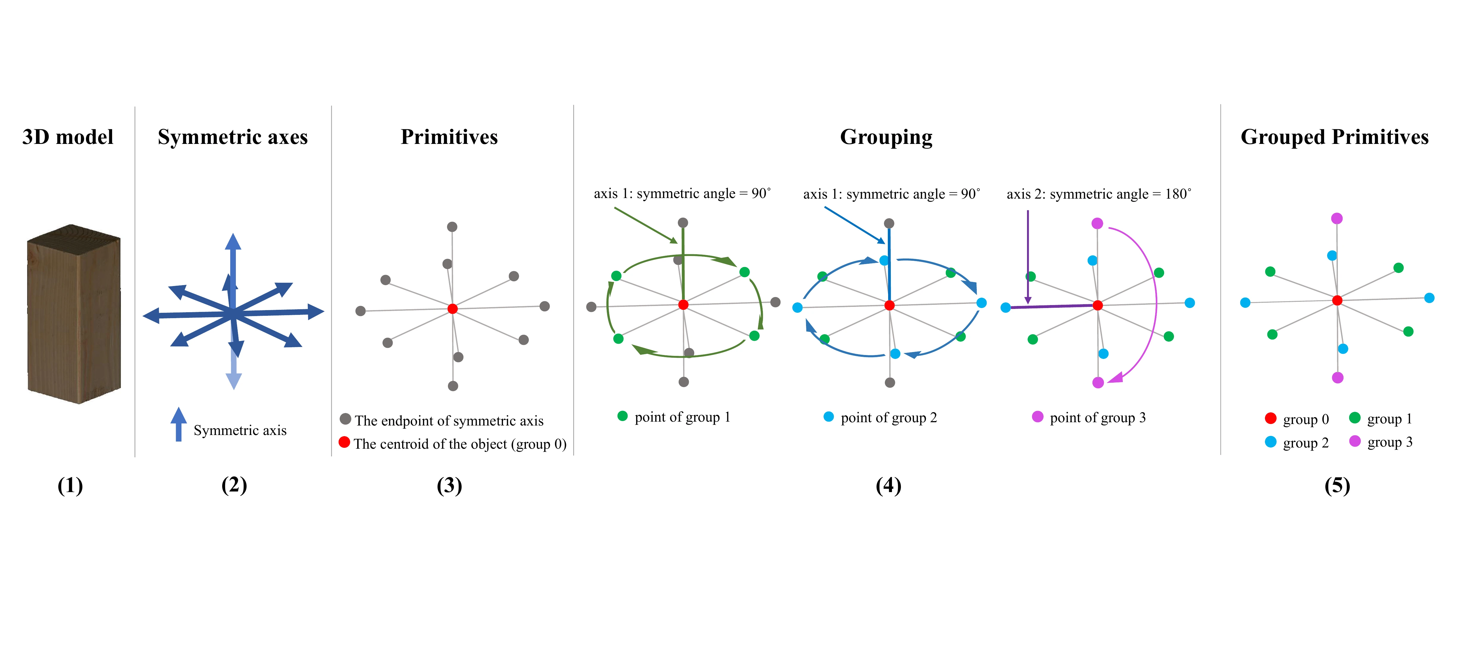
Figure 3. The pipeline of the GP construction.

Grouped primitives：我们在图3中展示了分组基元（GP）构建的流程。有了特定物体的三维模型后，我们可以根据公式\(\eqref{eq9}\)和\(\eqref{eq10}\)计算出所有的对称轴。用于分组的基元由对称轴的端点和物体质心组成。具体来说，需要以下三个步骤。

Step 1：这里定义并解释了对称轴-轴角的基本性质。物体\(O\)绕轴\(\boldsymbol{e} = (e_x, e_y, e_z)\)旋转角度\(\theta\)后外观保持不变，那么轴\(\boldsymbol{e}\)就是物体\(O\)的一条对称轴。轴\(\boldsymbol{e}\)和角度\(\theta\)构成了一个对称轴-轴角\(\boldsymbol{a}\)，其定义如下：

\[ \begin{equation}\label{eq7} \boldsymbol{a} = (\boldsymbol{e}, \theta), \quad \Vert\boldsymbol{e}\Vert = 1 \wedge \theta \in \{\frac{2\pi}{i}\}_{i = 2}^M. \end{equation} \]

需要注意的是，\(2\pi\)必须是对称角度\(\theta\)的整数倍（Symmetry），并且对称轴-轴角\(\boldsymbol{a}\)的阶数可以定义为：

\[ \begin{equation}\label{eq8} |\boldsymbol{a}| = \frac{2\pi}{\theta}(\boldsymbol{a}). \end{equation} \]

Figure 4. Grouped primitives and the visualization of A(M)GPD landscape. Based on the size of AO and ACO, symmetric objects can be classified into five categories. For each category, a typical toy model and its grouped primitives are presented in the first row plots. The second row shows the A(M)GPD landscape of each object in the rotation space, where the darker color represents the smaller value of A(M)GPD. The third row shows the minima in each landscape. Best viewed in color.

对称轴-轴角是一种冗余的表示形式。例如，对于图4中类别2的物体，如金字塔，它有四个对称轴-轴角：\((\boldsymbol{e}, \frac{\pi}{2})\)、\((\boldsymbol{e}, \pi)\)、\((-\boldsymbol{e}, \frac{\pi}{2})\)和\((-\boldsymbol{e}, \pi)\)，其中\(\boldsymbol{e}\)与绿色线条平行。在这种情况下，由于对称轴\(\boldsymbol{e}\)相同，这四个对称轴-轴角对于该物体而言具有相同的含义。由于旋转对称的周期性，这四个对称轴-轴角的角度必定存在最大公约数\(\frac{\pi}{2}\)。需要注意的是，在本研究中仅使用角度为最大公约数的对称轴-轴角，例如\((\boldsymbol{e}, \frac{\pi}{2})\)和\((-\boldsymbol{e}, \frac{\pi}{2})\)。

Step 2：在以物体质心为原点的物体坐标系中，可以通过使用以下公式得到物体\(O\)的一组粗略的对称轴-轴角：

\[ \begin{equation}\label{eq9} \hat{A}_O = \{\boldsymbol{a}|h(P_O, R(\boldsymbol{a})P_O) < \epsilon\}, \end{equation} \]

其中\(h\)是Hausdorff距离，\(P_O\)表示物体模型的顶点，\(R(\mathbf{a})\)是对称轴-轴角\(\mathbf{a}\)对应的旋转矩阵，并且允许的偏差由\(\varepsilon\)界定。然后，基于这些对称轴，应用MeanShift clustering algorithm（来自“Mean shift: a robust approach toward feature space analysis”）来简化\(\hat{A}_O\)：

\[ \begin{equation}\label{eq10} A_O = Mean\_Shift(\hat{A}_O), \end{equation} \]

此时，\(A_O\)包含了物体\(O\)的所有无冗余的对称轴-轴角，其中\(|A_O|\)是\(A_O\)的大小，且为\(2\)的倍数，因为对称轴-轴角总是成对出现，例如\((\mathbf{e}, \frac{\pi}{2})\)和\((-\mathbf{e}, \frac{\pi}{2})\)。此外，可以得到\(A_O\)的一个子集\(AC_{O}\)如下：

\[ \begin{equation}\label{eq11} AC_O = \{\boldsymbol{a} | \boldsymbol{a} \in A_O \wedge |\boldsymbol{a}| > \rho\}, \end{equation} \]

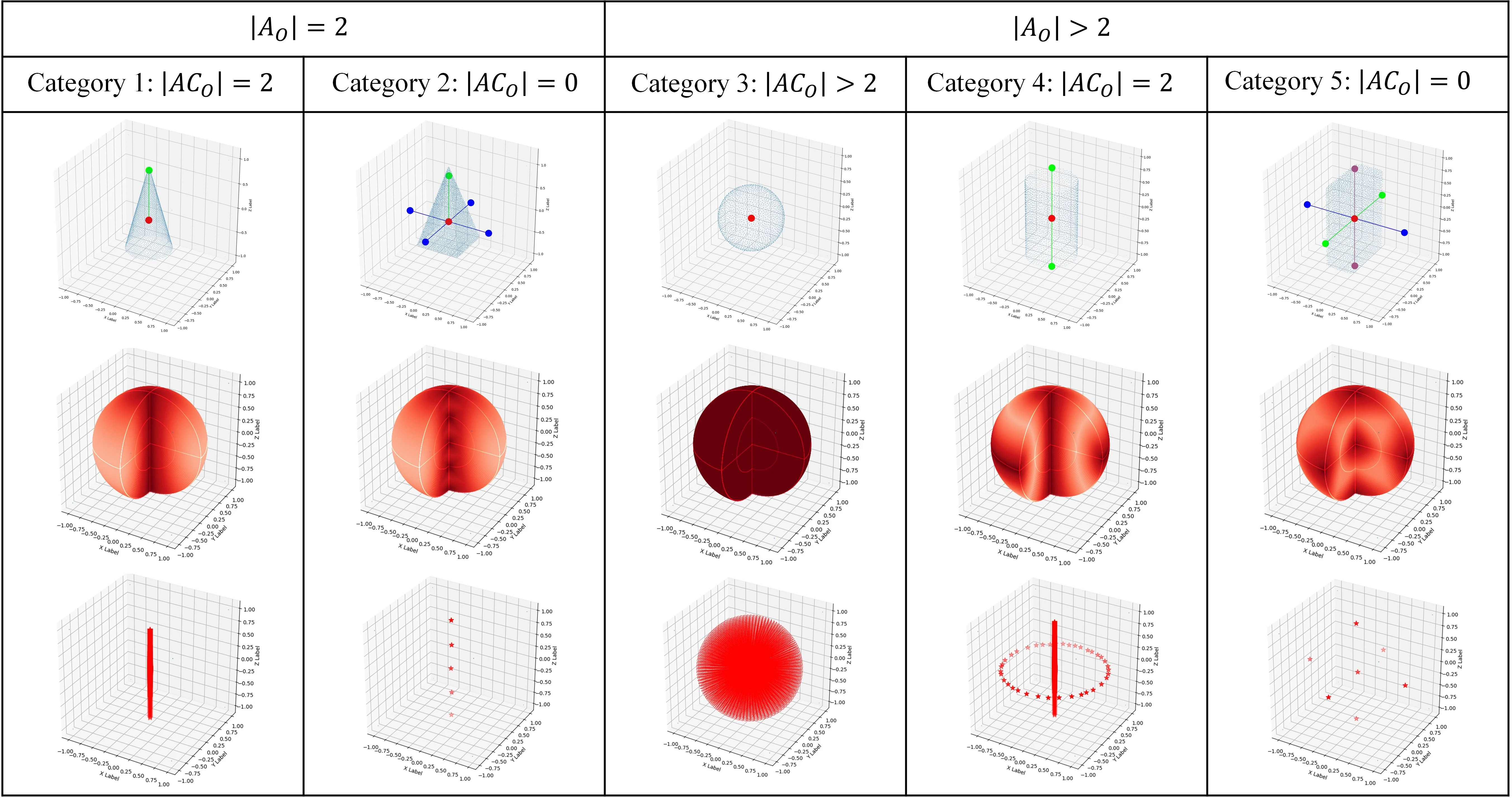
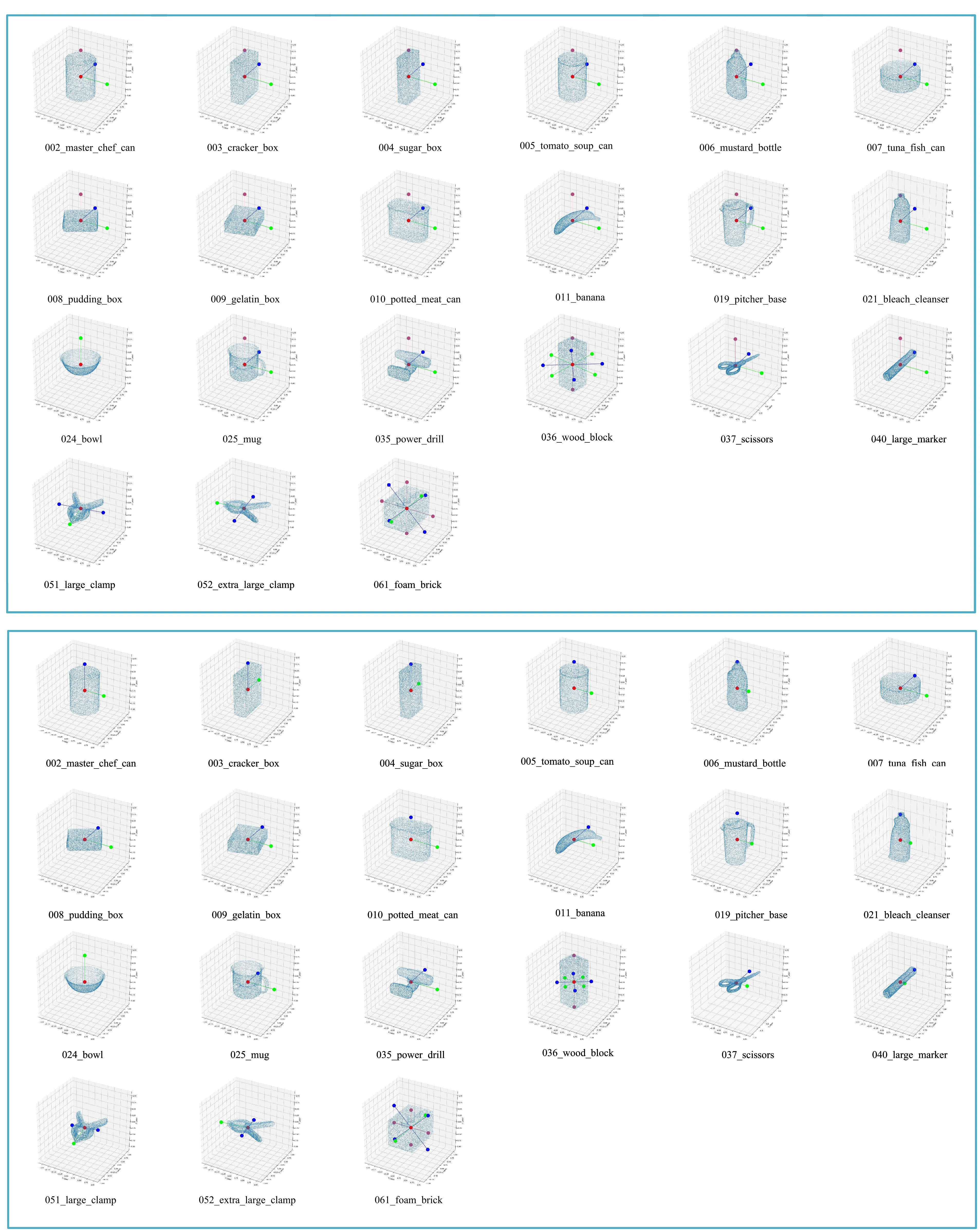
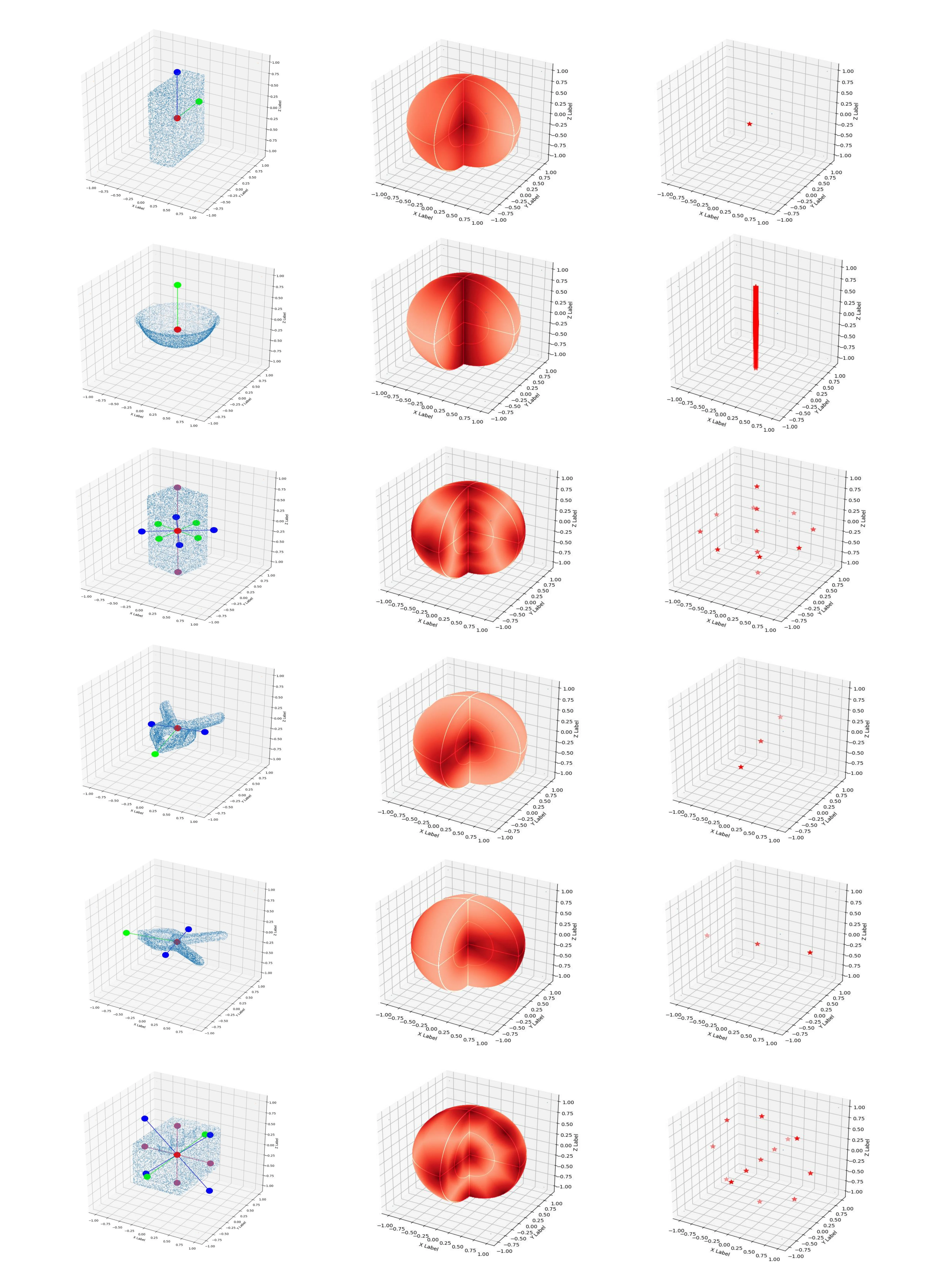
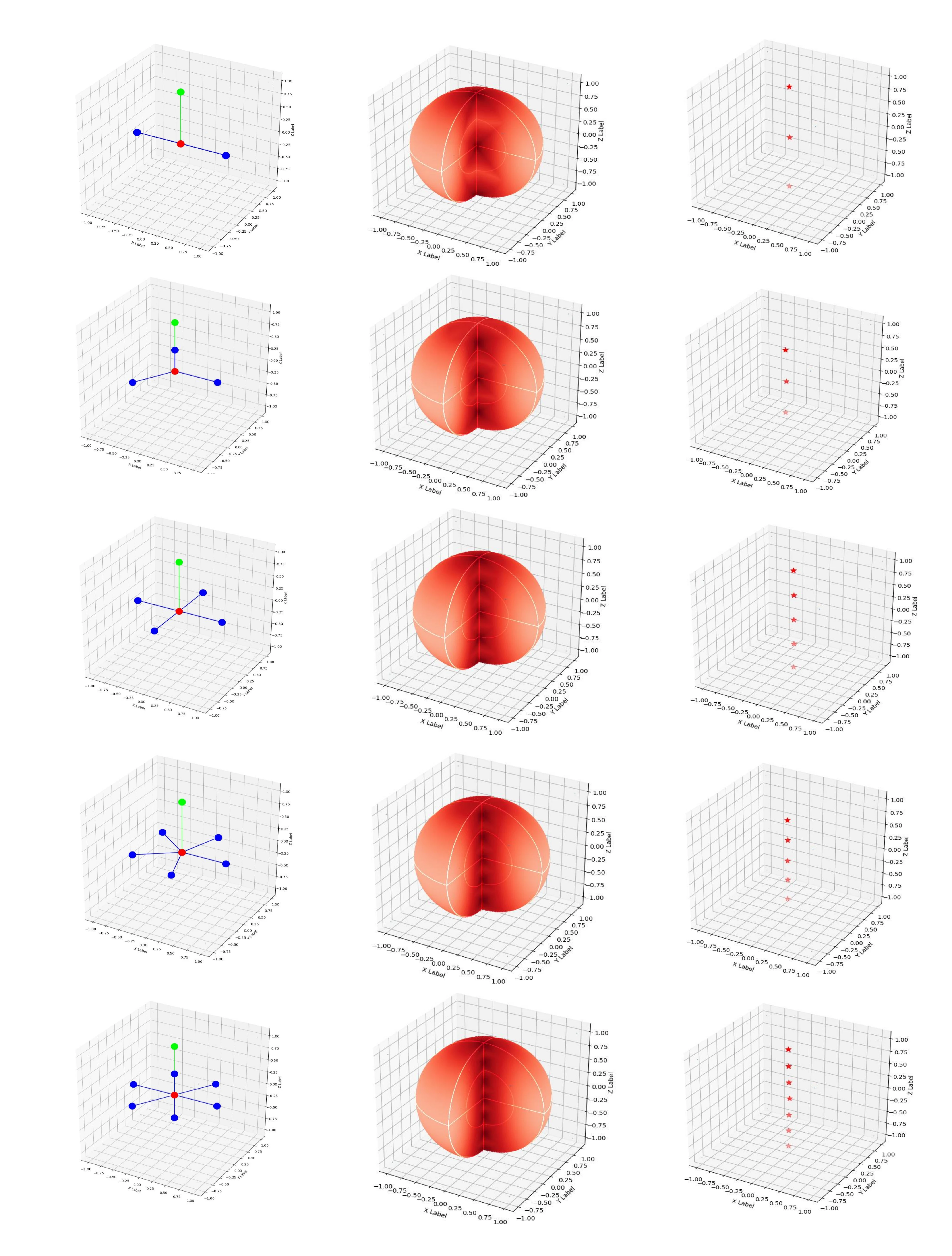
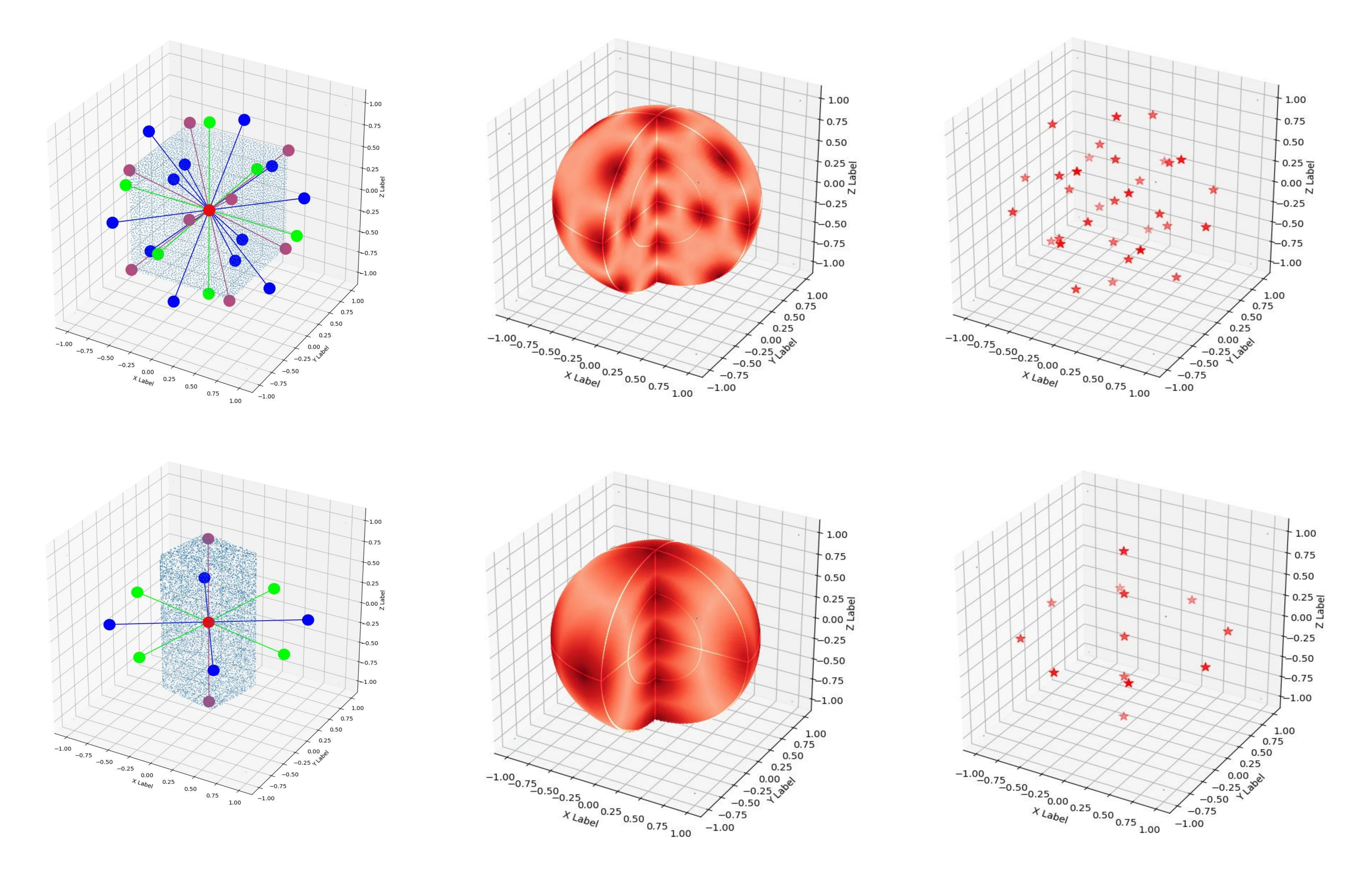
其中\(\rho\)是松弛阈值。当\(|\boldsymbol{a}| > \rho\)时，我们将\(\boldsymbol{a}\)视为连续的对称轴-轴角，并且当\(\rho\)设置为\(6\)时，涵盖了大多数应用情况，包括实验部分中要评估的所有物体。根据\(A_O\)和\(AC_O\)的大小，对称物体可以分为五类，如图4所示。

Step 3：如图3所示，如果基元\(A\)绕对称轴旋转特定角度后能够与基元\(B\)重合，那么我们就认为基元\(A\)和\(B\)属于同一组。分组后的基元记为\(G = \{g_i\}_{i = 0}^K\)，其中\(K\)是集合\(G\)的大小。分组原则的详细内容见补充材料。

Pose distance metric：基于分组基元（GP），设计了位姿距离度量A(M)GPD。A(M)GPD包含两个函数，第一个函数是平均分组基元距离（AGPD）：

\[ \begin{equation}\label{eq12} AGPD = \text{mean}_{g_i \in G}\ \text{mean}_{p_j \in g_i}\ \min_{p_k \in g_i, k \ne j} \Vert \hat{p}_j - \dot{p}_k \Vert, \end{equation} \]

其中\(\hat{p} = \hat{T}p\)，\(\dot{p} = \dot{T}p\)，\(p \in g(G)\)，并且\(\hat{T}\)，\(\dot{T} \in SE(3)\)。当物体\(O\)属于对称类别\(\{1, 3, 4, 5\}\)中的一个或者是非对称物体时，平均分组基元距离（AGPD）用于度量物体\(O\)的两个位姿之间的距离。

第2类与其他类别不同。它只有一对对称轴，且这对对称轴具有有限的阶数。如果将平均分组基元距离（AGPD）用作损失函数，这种特性会在旋转空间中导致错误的最小值，如图1的第二行所示。为了解决这个问题，引入了第二个函数——最大分组基元距离（MGPD）：

\[ \begin{equation}\label{eq13} MGPD = \max_{g_i \in G} \max_{p_j \in g_i} \min_{p_k \in g_i, k \ne j} \Vert \hat{p}_j - \dot{p}_k \Vert. \end{equation} \]

Loss for regression training：我们回归框架的总损失与DenseFusion中的损失类似，不同之处在于，我们使用A(M)GPD来计算预测值与真实值之间的误差，而不是使用ADD(S)。

3.5. Validation of A(M)GPD

在本小节中，提出了一种数值计算与可视化方法，用于检验A(M)GPD是否满足引言中所述的要求（1）all minima in the loss surface are mapped to the correct poses。为了更清晰地了解A(M)GPD在\(R \in SO(3)\)上的情况，我们首先采用采样技术生成\(N\)个旋转\(RC = \{R_i\}_{i = 1}^N\)，这些旋转在\(R \in SO(3)\)上密集分布。其次，将单位矩阵\(I_{3 \times 3}\)视为真实值，而\(\dot{R} \in RC\)作为预测值。\(I_{3 \times 3}\)与\(\dot{R}\)之间的A(M)GPD可表示为\(\dot{d}\)。

\[ \begin{equation}\label{eq14} \dot{d} = \text{A(M)GPD}(I_{3 \times 3}, \dot{R}). \end{equation} \]

然后，我们借助旋转向量\(\boldsymbol{v} = (v_x, v_y, v_z)\)来可视化\(\dot{d}\)，其中向量的方向为旋转轴，长度为旋转角度\(\theta \in [0, \pi]\)。如图4中第二行的图所示，\(\dot{R}\)的坐标为\(\boldsymbol{v}(\dot{R})\)，\(\dot{R}\)的颜色值对应着相应的\(\dot{d}\)（颜色越深表示\(\dot{d}\)越小）。然而，在这些图中很难找到最小值，所以我们通过一个简单的算法进一步模拟梯度下降的过程。该算法的原理是\(\boldsymbol{v}(\dot{R})\)不断地向\(\boldsymbol{v}(\hat{R})\)移动，\(\boldsymbol{v}(\hat{R})\)在\(\boldsymbol{v}(\dot{R})\)的邻域内具有最小的\(\hat{d}\)，并且这个点最终会停在一个局部最小值处。我们对每个\(\boldsymbol{v}(\dot{R})\)都应用这个原理，并且在图4第三行的图中用红色星号标记出找到的最小值。如我们所见，所有的最小值都被映射到了正确的位姿上。其他物体的情况在补充材料中给出。