【论文笔记】Emerging Properties in Self-Supervised Vision Transformers
Emerging Properties in Self-Supervised Vision Transformers
![Figure 1: Self-attention from a Vision Transformer with 8 \times 8 patches trained with no supervision. We look at the self-attention of the [CLS] token on the heads of the last layer. This token is not attached to any label nor supervision. These maps show that the model automatically learns class-specific features leading to unsupervised object segmentations.](https://img.032802.xyz/paper-reading/2021/emerging-properties-in-self-supervised-vision-transformers_2021_Caron/attn6.webp)
Abstract
1. Introduction
2. Related Work
3. Approach
"Talk is cheap. Show me the code."
― Linus Torvalds
DINO的原仓库给出了一个demo:
1 | # Copyright (c) Facebook, Inc. and its affiliates. |
同时也给出了这段代码的运行方式:
1 | python visualize_attention.py |
我们不妨直接运行,其结果如下:
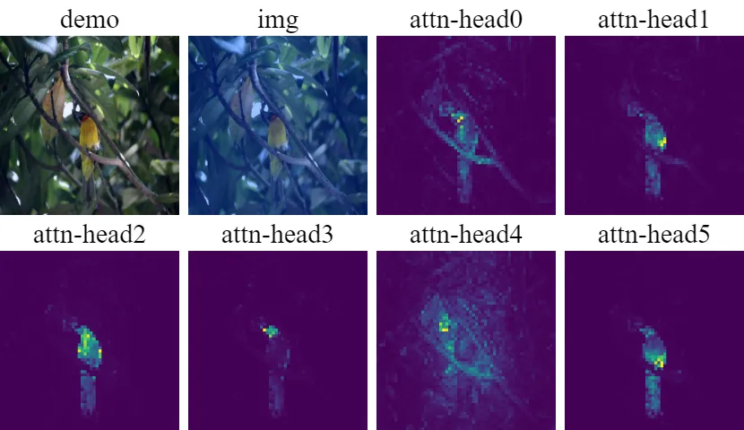
其中:
demo:表示输入图像;img:表示输入图像经过torchvision.utils.make_grid(img, normalize=True, scale_each=True)函数处理后的图像;attn-head0 - attn-head5:表示第0个注意力头到第5个注意力头的注意力图。
接下来我们逐行分析visualize_attention.py的代码:
1-35行:引入包;
38-41行:定义
apply_mask函数,该函数用于将彩色遮罩叠加到原始图像上;44-52行:定义
random_colors函数,该函数用于生成随机颜色,使用HSV颜色空间来确保生成的颜色具有良好的视觉区分度;55-95行:定义
display_instances函数,该函数用于显示和保存带有遮罩的图像;98-213行:
main函数,接下来会详细解释main函数:- 99-148行:接收参数、加载模型;
- 151-170行:读取图像,并对图像进行预处理;
- 173-174行:make the image divisible by the patch size;
- 176-177行:获取注意力图的高和宽;
- 179行:获取所有注意力头的注意力图;
- 181行:获取注意力头的数量;
- 184行:在所有注意力头上获取类别标签[CLS]对图像所有patch的注意力向量;
- 186-197行:如果传入了
--threshold参数,则只保留累积注意力值达到阈值的区域这里在运行demo时没有设置--threshold参数,所以没有执行这一段代码,th_attn为空; - 199-200行:在所有注意力头上将类别标签[CLS]对图像所有patch的注意力向量reshape成2维图像,假设有\(n\)个注意力头,那么此时有\(n\)个2维图像,在reshape后,使用最近邻
nearest插值将注意力图的分辨率恢复到输入图像的分辨率; - 203-208行:保存所有注意力头的注意力图;
- 210-213行:保存186-197行处理后的注意力图。
显然,179行的attentions = model.get_last_selfattention(img.to(device))是整段代码的关键。
get_last_selfattention函数的定义在vision_transformer.py第216行:
1 | class VisionTransformer(nn.Module): |
get_last_selfattention函数在执行时,首先会调用prepare_tokens函数,prepare_tokens函数的定义在vision_transformer.py第196行:
1 | class VisionTransformer(nn.Module): |
prepare_tokens函数在执行时,会继续调用patch_embed,patch_embed是PatchEmbed类的实例,PatchEmbed类的定义在vision_transformer.py第116行:
1 | class PatchEmbed(nn.Module): |
PatchEmbed类继承于nn.Module,所以先看forward函数:
B, C, H, W = x.shape是获取了图像的batch_size B、通道数C、图像高度H和图像宽度W;x = self.proj(x).flatten(2).transpose(1, 2)等价于顺序执行下面三步:x = self.proj(x),x = x.flatten(2),x = x.transpose(1, 2);其中:
x = self.proj(x)表示使用卷积核nn.Conv2d(in_chans, embed_dim, kernel_size=patch_size, stride=patch_size)对输入图像进行了处理,in_chans为输入通道数,embed_dim为输出通道数,kernel_size为卷积核大小,stride为步长。这里的embed_dim就是\(D\),patch_size就是\(P\),且该卷积操作的卷积核大小和步长大小相同,所以将输入图片经过这个卷积操作后,每一个patch都会被映射成一个\(D\)维的向量,且patch和patch之间没有重合部分,那么最后输出的维度是\(\mathbb{R}^{B \times D \times \frac{H}{P} \times \frac{W}{P}}\);x = x.flatten(2)表示从x的第2维开始展平,保持维度0和1不变,将维度2和3合并,令\(N = \frac{H}{P} \times \frac{W}{P}\)为patch的数量,那么最后输出的维度是\(\mathbb{R}^{B \times D \times N}\);x = x.transpose(1, 2)表示将维度1和维度2交换,那么最后输出的维度是\(\mathbb{R}^{B \times N \times D}\),用卷积核的参数表示,输出的维度为\(\mathbb{R}^{B \times \frac{\text{img_size}^2}{\text{patch_size}^2} \times \text{embed_dim}}\)。
patch_embed类结束,回到prepare_tokens函数:
1 | class VisionTransformer(nn.Module): |
在执行完x = self.patch_embed(x)后,x的维度为\(\mathbb{R}^{B \times
\frac{\text{img_size}^2}{\text{patch_size}^2} \times
\text{embed_dim}}\),self.cls_token的维度为\(\mathbb{R}^{1 \times 1 \times
\text{embed_dim}}\),所以在expand(B, -1, -1)之后,cls_tokens的维度为\(\mathbb{R}^{B \times 1 \times
\text{embed_dim}}\),x = torch.cat((cls_tokens, x), dim=1)表示将cls_tokens和x在第1维上拼接,那么最后x的维度为\(\mathbb{R}^{B \times
\left(\frac{\text{img_size}^2}{\text{patch_size}^2} + 1\right) \times
\text{embed_dim}}\)。
reshape做完,线性映射完,[CLS]拼接完,接下来是位置编码,即x = x + self.interpolate_pos_encoding(x, w, h),interpolate_pos_encoding函数的定义在vision_transformer.py第174行:
1 | class VisionTransformer(nn.Module): |
简单来说,这个函数能够基于初始化生成的位置编码,用插值的方法为不同分辨率的输入图像生成对应的位置编码,以让模型能够处理不同尺寸的输入图像。
最后,返回self.pos_drop(x),pos_drop函数就是一个简单的nn.Dropout,所以最后x的维度为\(\mathbb{R}^{B \times
\left(\frac{\text{img_size}^2}{\text{patch_size}^2} + 1\right) \times
\text{embed_dim}}\)。
prepare_tokens函数结束,回到get_last_selfattention函数:
1 | class VisionTransformer(nn.Module): |
简单来说,在准备完tokens即x = self.prepare_tokens(x)执行结束后,让x逐个通过所有的self.blocks,当到达最后一个block时,返回最后一个block的注意力图。
那么现在需要知道self.blocks是什么,self.blocks是一个nn.ModuleList,其中包含depth个Block类,Block类的定义在vision_transformer.py第95行:
1 | class Block(nn.Module): |
Block类的核心部分便是Attention类,而Attention类的定义在vision_transformer.py第68行:
1 | class Attention(nn.Module): |
在这个Attention类中,同时实现了单头注意力和多头注意力,逐行进行分析:
def __init__(self, dim, num_heads=8, qkv_bias=False, qk_scale=None, attn_drop=0., proj_drop=0.):super().__init__():调用父类nn.Module的构造函数;self.num_heads = num_heads:设置注意力头的数量;head_dim = dim // num_heads:设置每个注意力头所需要处理的特征维度;self.scale = qk_scale or head_dim ** -0.5:设置注意力分数的缩放因子,如果qk_scale不为空,则使用qk_scale,否则使用head_dim的负0.5次方作为缩放因子,即\(\frac{1}{\sqrt{\text{head_dim}}}\),和原版Transformer中的设置一致;self.qkv = nn.Linear(dim, dim * 3, bias=qkv_bias):定义一个线性层,将原本的特征维度从C变为3 * C,以便于在后续切分为q,k,v;self.attn_drop = nn.Dropout(attn_drop):注意力Dropout;self.proj = nn.Linear(dim, dim):一个线性层;self.proj_drop = nn.Dropout(proj_drop):投影Dropout;
def forward(self, x):B, N, C = x.shape:获取输入张量的维度,B表示批量大小,N表示序列长度,C表示特征维度,也就是说\(\mathbf{x} \in \mathbb{R}^{B \times N \times C}\);qkv = self.qkv(x).reshape(B, N, 3, self.num_heads, C // self.num_heads).permute(2, 0, 3, 1, 4):等价于顺序执行下面三步:qkv = self.qkv(x),qkv = qkv.reshape(B, N, 3, self.num_heads, C // self.num_heads),qkv = qkv.permute(2, 0, 3, 1, 4);其中:
qkv = self.qkv(x):\(\mathbf{qkv} \in \mathbb{R}^{B \times N \times 3C}\);qkv = qkv.reshape(B, N, 3, self.num_heads, C // self.num_heads):\(\mathbf{qkv} \in \mathbb{R}^{B \times N \times 3 \times \text{num_heads} \times \frac{C}{\text{num_heads}}}\);qkv = qkv.permute(2, 0, 3, 1, 4):\(\mathbf{qkv} \in \mathbb{R}^{3 \times B \times \text{num_heads} \times N \times \frac{C}{\text{num_heads}}}\);
q, k, v = qkv[0], qkv[1], qkv[2]:- \(\mathbf{q} \in \mathbb{R}^{B \times \text{num_heads} \times N \times \frac{C}{\text{num_heads}}}\);
- \(\mathbf{k} \in \mathbb{R}^{B \times \text{num_heads} \times N \times \frac{C}{\text{num_heads}}}\);
- \(\mathbf{v} \in \mathbb{R}^{B \times \text{num_heads} \times N \times \frac{C}{\text{num_heads}}}\);
attn = (q @ k.transpose(-2, -1)) * self.scale:\(\mathbf{attn} \in \mathbb{R}^{B \times \text{num_heads} \times N \times N}\);attn = attn.softmax(dim=-1):softmax归一化;attn = self.attn_drop(attn):注意力Dropout;x = (attn @ v).transpose(1, 2).reshape(B, N, C):等价于顺序执行下面三步:x = (attn @ v),x = x.transpose(1, 2),x = x.reshape(B, N, C);其中:
x = (attn @ v):\(\mathbf{x} \in \mathbb{R}^{B \times \text{num_heads} \times N \times \frac{C}{\text{num_heads}}}\);x = x.transpose(1, 2):\(\mathbf{x} \in \mathbb{R}^{B \times N \times \text{num_heads} \times \frac{C}{\text{num_heads}}}\);x = x.reshape(B, N, C):\(\mathbf{x} \in \mathbb{R}^{B \times N \times C}\);
x = self.proj(x):\(\mathbf{x} \in \mathbb{R}^{B \times N \times C}\);x = self.proj_drop(x):投影Dropout;return x, attn:- \(\mathbf{x} \in \mathbb{R}^{B \times N \times C}\);
- \(\mathbf{attn} \in \mathbb{R}^{B \times \text{num_heads} \times N \times N}\)。
Attention类结束,回到Block类:
1 | class Block(nn.Module): |
Block类中关键的就只有self.attn了,所以不详细介绍了,要注意的是在forward中,当return_attention=True时,返回的是注意力图,否则返回的是输入经过注意力机制后的结果。
Block类结束,回到get_last_selfattention函数,get_last_selfattention函数中只是Block类的堆叠,所以get_last_selfattention函数也结束。
vision_transformer.py文件中还有下面几个部分没有提到:
drop_path函数:该函数值得展开,函数定义在vision_transformer.py第27行:
1
2
3
4
5
6
7
8
9def drop_path(x, drop_prob: float = 0., training: bool = False):
if drop_prob == 0. or not training:
return x
keep_prob = 1 - drop_prob
shape = (x.shape[0],) + (1,) * (x.ndim - 1) # work with diff dim tensors, not just 2D ConvNets
random_tensor = keep_prob + torch.rand(shape, dtype=x.dtype, device=x.device)
random_tensor.floor_() # binarize
output = x.div(keep_prob) * random_tensor
return outputdrop_path,顾名思义,就是丢弃一整条路径上的所有值,但是实际上,drop_path是丢弃输入向量中的若干分量:if drop_prob == 0. or not training: return x:如果drop_prob为0,或者训练模式为False,则直接返回输入向量;keep_prob = 1 - drop_prob:计算保留的概率;shape = (x.shape[0],) + (1,) * (x.ndim - 1):创建一个与输入张量兼容的广播形状,保持第一维(批次维)不变,其他维度都设为1;random_tensor = keep_prob + torch.rand(shape, dtype=x.dtype, device=x.device):生成一个与输入张量兼容的随机张量,其值在[0 + keep_prob, 1 + keep_prob]之间;random_tensor.floor_():将随机张量的值向下取整为0或1,相当于二值化;output = x.div(keep_prob) * random_tensor:将输入张量除以保留概率,然后与二值化后的随机张量相乘,得到输出张量;return output:返回输出张量;DropPath与Dropout相比,能够通过缩放保持期望值不变,提供了更好的正则化效果,帮助网络学习更鲁棒的特征;
DropPath类:使用drop_path函数处理输入的向量;Mlp类:在Block类中使用到的MLP层;vit_tiny函数:1
2
3
4
5def vit_tiny(patch_size=16, **kwargs):
model = VisionTransformer(
patch_size=patch_size, embed_dim=192, depth=12, num_heads=3, mlp_ratio=4,
qkv_bias=True, norm_layer=partial(nn.LayerNorm, eps=1e-6), **kwargs)
return modelmlp_ratio=4:MLP隐藏层维度是嵌入维度的4倍,比如这里MLP隐藏层的维度就是192 * 4 = 768;
vit_small函数:embed_dim=384;num_heads=6;
vit_base函数:embed_dim=768;num_heads=12;
DINOHead类:DINO自监督学习中的特征投影,用于计算学生和教师网络输出的相似度。
还没完,VisionTransformer类中还有下面几个函数没有提到:
_init_weights函数:针对不同的层采取不同的初始化方案;forward函数:只输出[CLS] token,用于分类任务;get_intermediate_layers函数:用于获取Vision Transformer最后n个块的中间层特征。
3.1. SSL with Knowledge Distillation
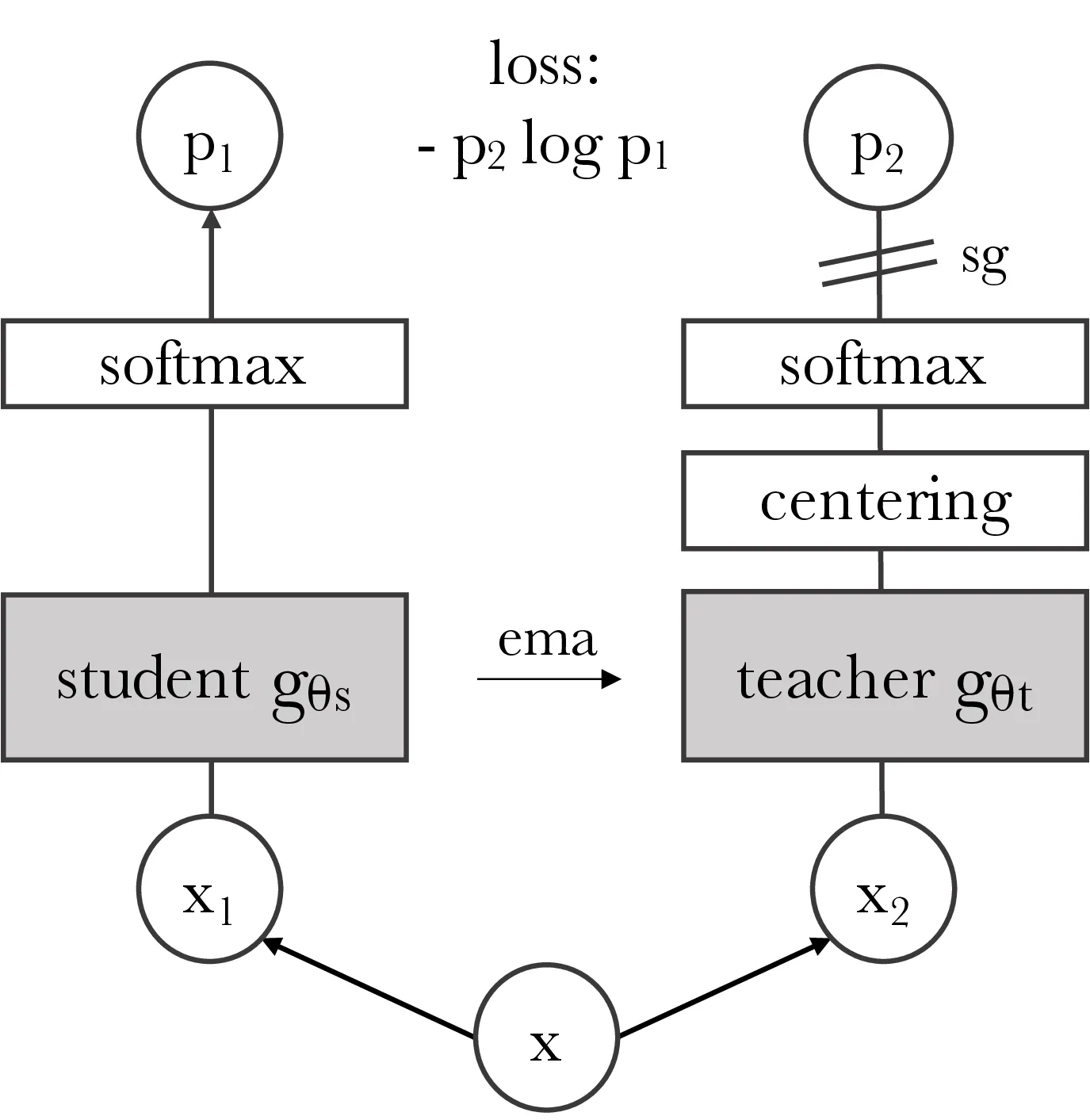
Algorithm 1 DINO PyTorch pseudocode w/o multi-crop.

# gs, gt: student and teacher networks
# C: center (K)
# tps, tpt: student and teacher temperatures
# l, m: network and center momentum rates
gt.params = gs.params
for x in loader: # load a minibatch x with n samples
    x1, x2 = augment(x), augment(x) # random views

    s1, s2 = gs(x1), gs(x2) # student output n-by-K
    t1, t2 = gt(x1), gt(x2) # teacher output n-by-K

    loss = H(t1, s2)/2 + H(t2, s1)/2
    loss.backward() # back-propagate

    # student, teacher and center updates
    update(gs) # SGD
    gt.params = l*gt.params + (1-l)*gs.params
    C = m*C + (1-m)*cat([t1, t2]).mean(dim=0)

def H(t, s):
    t = t.detach() # stop gradient
    s = softmax(s / tps, dim=1)
    t = softmax((t - C) / tpt, dim=1) # center + sharpen
    return - (t * log(s)).sum(dim=1).mean()
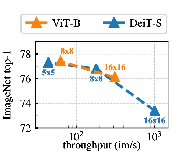
3.2. Implementation and evaluation protocols
| model | blocks | dim | heads | #tokens | #params | im/s |
|---|---|---|---|---|---|---|
| ResNet-50 | - | 2048 | - | - | 23M | 1237 |
| ViT-S/16 | 12 | 384 | 6 | 197 | 21M | 1007 |
| ViT-S/8 | 12 | 384 | 6 | 785 | 21M | 180 |
| ViT-B/16 | 12 | 768 | 12 | 197 | 85M | 312 |
| ViT-B/8 | 12 | 768 | 12 | 785 | 85M | 63 |
4. Main Results
4.1. Comparing with SSL frameworks on ImageNet
| Method | Arch. | Param. | im/s | Linear | \(k\)-NN |
|---|---|---|---|---|---|
| Supervised | RN50 | 23 | 1237 | 79.3 | 79.3 |
| SCLR [12] | RN50 | 23 | 1237 | 69.1 | 60.7 |
| MoCov2 [15] | RN50 | 23 | 1237 | 71.1 | 61.9 |
| InfoMin [67] | RN50 | 23 | 1237 | 73.0 | 65.3 |
| BarlowT [81] | RN50 | 23 | 1237 | 73.2 | 66.0 |
| OBoW [27] | RN50 | 23 | 1237 | 73.8 | 61.9 |
| BYOL [30] | RN50 | 23 | 1237 | 74.4 | 64.8 |
| DCv2 [10] | RN50 | 23 | 1237 | 75.2 | 67.1 |
| SwAV [10] | RN50 | 23 | 1237 | 75.3 | 65.7 |
| DINO | RN50 | 23 | 1237 | 75.3 | 67.5 |
| Supervised | ViT-S | 21 | 1007 | 79.8 | 79.8 |
| BYOL∗ [30] | ViT-S | 21 | 1007 | 71.4 | 66.6 |
| MoCov2∗ [15] | ViT-S | 21 | 1007 | 72.7 | 64.4 |
| SwAV∗ [10] | ViT-S | 21 | 1007 | 73.5 | 66.3 |
| DINO | ViT-S | 21 | 1007 | 77.0 | 74.5 |
| Comparison across architectures | |||||
| SCLR [12] | RN50w4 | 375 | 117 | 76.8 | 69.3 |
| SwAV [10] | RN50w2 | 93 | 384 | 77.3 | 67.3 |
| BYOL [30] | RN50w2 | 93 | 384 | 77.4 | - |
| DINO | ViT-B/16 | 85 | 312 | 78.2 | 76.1 |
| SwAV [10] | RN50w5 | 586 | 76 | 78.5 | 67.1 |
| BYOL [30] | RN50w4 | 375 | 117 | 78.6 | - |
| BYOL [30] | RN200w2 | 250 | 123 | 79.6 | 73.9 |
| DINO | ViT-S/8 | 21 | 180 | 79.7 | 78.3 |
| SCLRv2 [13] | RN152w3+SK | 794 | 46 | 79.8 | 73.1 |
| DINO | ViT-B/8 | 85 | 63 | 80.1 | 77.4 |
4.2. Properties of ViT trained with SSL
4.2.1 Nearest neighbor retrieval with DINO ViT
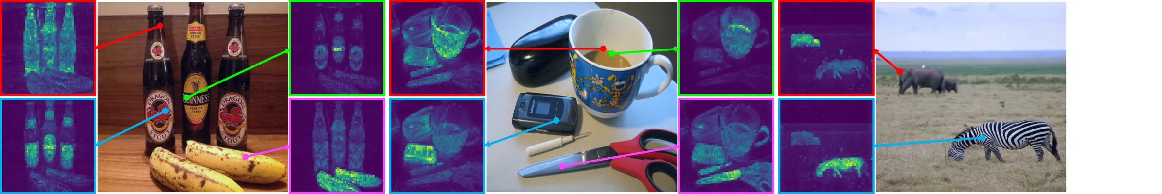
![Figure 3: Attention maps from multiple heads. We consider the heads from the last layer of a ViT-S/8 trained with DINO and display the self-attention for [CLS] token query. Different heads, materialized by different colors, focus on different locations that represents different objects or parts (more examples in Appendix).](https://img.032802.xyz/paper-reading/2021/emerging-properties-in-self-supervised-vision-transformers_2021_Caron/fig3.webp)
| Pretrain | Arch. | Pretrain | \(\mathcal{R}\)Ox | \(\mathcal{R}\)Par | ||
|---|---|---|---|---|---|---|
| M | H | M | H | |||
| Sup. [57] | RN101+R-MAC | ImNet | 49.8 | 18.5 | 74.0 | 52.1 |
| Sup. | ViT-S/16 | ImNet | 33.5 | 8.9 | 63.0 | 37.2 |
| DINO | ResNet-50 | ImNet | 35.4 | 11.1 | 55.9 | 27.5 |
| DINO | ViT-S/16 | ImNet | 41.8 | 13.7 | 63.1 | 34.4 |
| DINO | ViT-S/16 | GLDv2 | 51.5 | 24.3 | 75.3 | 51.6 |
| Method | Arch. | Dim. | Resolution | mAP |
|---|---|---|---|---|
| Multigrain [5] | ResNet-50 | 2048 | 2242 | 75.1 |
| Multigrain [5] | ResNet-50 | 2048 | largest side 800 | 82.5 |
| Supervised [69] | ViT-B/16 | 1536 | 2242 | 76.4 |
| DINO | ViT-B/16 | 1536 | 2242 | 81.7 |
| DINO | ViT-B/8 | 1536 | 3202 | 85.5 |
| Method | Data | Arch. | \((\mathcal{J}\&\mathcal{F})_m\) | \(\mathcal{J}_m\) | \(\mathcal{F}_m\) |
|---|---|---|---|---|---|
| Supervised | |||||
| ImageNet | INet | ViT-S/8 | 66.0 | 63.9 | 68.1 |
| STM [48] | I/D/Y | RN50 | 81.8 | 79.2 | 84.3 |
| Self-supervised | |||||
| CT [71] | VLOG | RN50 | 48.7 | 46.4 | 50.0 |
| MAST [40] | YT-VOS | RN18 | 65.5 | 63.3 | 67.6 |
| STC [37] | Kinetics | RN18 | 67.6 | 64.8 | 70.2 |
| DINO | INet | ViT-S/16 | 61.8 | 60.2 | 63.4 |
| DINO | INet | ViT-B/16 | 62.3 | 60.7 | 63.9 |
| DINO | INet | ViT-S/8 | 69.9 | 66.6 | 73.1 |
| DINO | INet | ViT-B/8 | 71.4 | 67.9 | 74.9 |
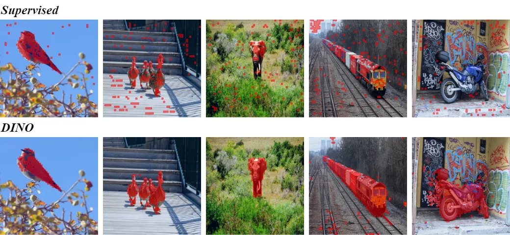
4.2.2 Discovering the semantic layout of scenes
4.2.3 Transfer learning on downstream tasks
5. Ablation Study of DINO
5.1. Importance of the Different Components
| Random | Supervised | DINO | |
|---|---|---|---|
| ViT-S/16 | 22.0 | 27.3 | 45.9 |
| ViT-S/8 | 21.8 | 23.7 | 44.7 |
| Cifar10 | Cifar100 | INat18 | INat19 | Flwrs | Cars | INet | |
|---|---|---|---|---|---|---|---|
| ViT-S/16 | |||||||
| Sup. [69] | 99.0 | 89.5 | 70.7 | 76.6 | 98.2 | 92.1 | 79.9 |
| DINO | 99.0 | 90.5 | 72.0 | 78.2 | 98.5 | 93.0 | 81.5 |
| ViT-B/16 | |||||||
| Sup. [69] | 99.0 | 90.8 | 73.2 | 77.7 | 98.4 | 92.1 | 81.8 |
| DINO | 99.1 | 91.7 | 72.6 | 78.6 | 98.8 | 93.0 | 82.8 |
| Method | Mom. | SK | MC | Loss | Pred. | \(k\)-NN | Lin. | |
|---|---|---|---|---|---|---|---|---|
| 1 | DINO | ✓ | ✗ | ✓ | CE | ✗ | 72.8 | 76.1 |
| 2 | ✗ | ✗ | ✓ | CE | ✗ | 0.1 | 0.1 | |
| 3 | ✓ | ✓ | ✓ | CE | ✗ | 72.2 | 76.0 | |
| 4 | ✓ | ✗ | ✗ | CE | ✗ | 67.9 | 72.5 | |
| 5 | ✓ | ✗ | ✓ | MSE | ✗ | 52.6 | 62.4 | |
| 6 | ✓ | ✗ | ✓ | CE | ✓ | 71.8 | 75.6 | |
| 7 | BYOL | ✓ | ✗ | ✗ | MSE | ✓ | 66.6 | 71.4 |
| 8 | MoCov2 | ✓ | ✗ | ✗ | INCE | ✗ | 62.0 | 71.6 |
| 9 | SwAV | ✗ | ✓ | ✓ | CE | ✗ | 64.7 | 71.8 |
|
SK: Sinkhorn-Knopp, MC: Multi-Crop, Pred.: Predictor CE: Cross-Entropy, MSE: Mean Square Error, INCE: InfoNCE |
||||||||
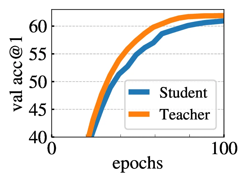
5.2. Impact of the choice of Teacher Network
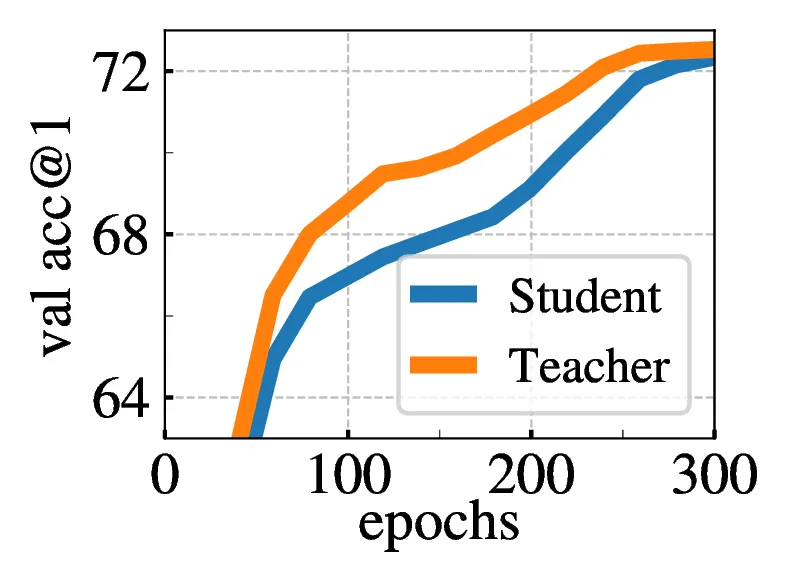
| Teacher | Top-1 |
|---|---|
| Student copy | 0.1 |
| Previous iter | 0.1 |
| Previous epoch | 66.6 |
| Momentum | 72.8 |
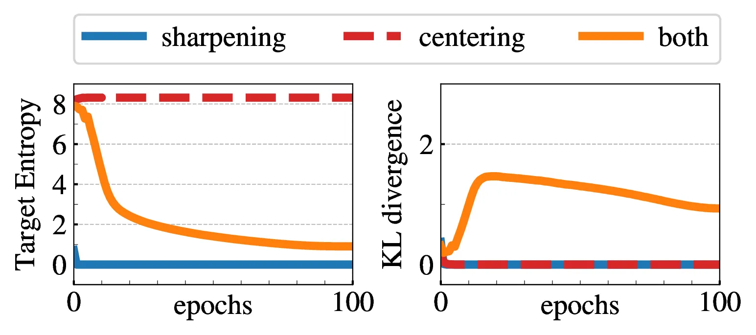
5.3. Avoiding collapse
| multi-crop | 100 epochs | 300 epochs | mem. | ||
|---|---|---|---|---|---|
| top-1 | time | top-1 | time | ||
| 2 × 2242 | 67.8 | 15.3h | 72.5 | 45.9h | 9.3G |
| 2 × 2242 + 2 × 962 | 71.5 | 17.0h | 74.5 | 51.0h | 10.5G |
| 2 × 2242 + 6 × 962 | 73.8 | 20.3h | 75.9 | 60.9h | 12.9G |
| 2 × 2242 + 10 × 962 | 74.6 | 24.2h | 76.1 | 72.6h | 15.4G |
5.4. Compute requirements
5.5. Training with small batches
| bs | 128 | 256 | 512 | 1024 |
|---|---|---|---|---|
| top-1 | 57.9 | 59.1 | 59.6 | 59.9 |
Appendix
A. Additional Results
| Logistic | \(k\)-NN | |||||
|---|---|---|---|---|---|---|
| RN50 | ViT-S | \(\Delta\) | RN50 | ViT-S | \(\Delta\) | |
| Inet 100% | 72.1 | 75.7 | 3.6 | 67.5 | 74.5 | 7.0 |
| Inet 10% | 67.8 | 72.2 | 4.4 | 59.3 | 69.1 | 9.8 |
| Inet 1% | 55.1 | 64.5 | 9.4 | 47.2 | 61.3 | 14.1 |
| Pl. 10% | 53.4 | 52.1 | -1.3 | 46.9 | 48.6 | 1.7 |
| Pl. 1% | 46.5 | 46.3 | -0.2 | 39.2 | 41.3 | 2.1 |
| VOC07 | 88.9 | 89.2 | 0.3 | 84.9 | 88.0 | 3.1 |
| FLOWERS | 95.6 | 96.4 | 0.8 | 87.9 | 89.1 | 1.2 |
| Average \(\Delta\) | 2.4 | 5.6 | ||||
| Pretraining | res. | tr. proc. | Top-1 | |
|---|---|---|---|---|
| method | data | |||
| Pretrain on additional data | ||||
| MMP | JFT-300M | 384 | [19] | 79.9 |
| Supervised | JFT-300M | 384 | [19] | 84.2 |
| Train with additional model | ||||
| Rand. init. | - | 224 | [69] | 83.4 |
| No additional data nor model | ||||
| Rand. init. | - | 224 | [19] | 77.9 |
| Rand. init. | - | 224 | [69] | 81.8 |
| Supervised | ImNet | 224 | [69] | 81.9 |
| DINO | ImNet | 224 | [69] | 82.8 |
| Method | Arch | Param. | Top 1 | |
|---|---|---|---|---|
| 1% | 10% | |||
| Self-supervised pretraining with finetuning | ||||
| UDA [75] | RN50 | 23 | - | 68.1 |
| SimCLRv2 [13] | RN50 | 23 | 57.9 | 68.4 |
| BYOL [30] | RN50 | 23 | 53.2 | 68.8 |
| SwAV [10] | RN50 | 23 | 53.9 | 70.2 |
| SimCLRv2 [16] | RN50w4 | 375 | 63.0 | 74.4 |
| BYOL [30] | RN200w2 | 250 | 71.2 | 77.7 |
| Semi-supervised methods | ||||
| SimCLRv2+KD [13] | RN50 | 23 | 60.0 | 70.5 |
| SwAV+CT [3] | RN50 | 23 | - | 70.8 |
| FixMatch [64] | RN50 | 23 | - | 71.5 |
| MPL [49] | RN50 | 23 | - | 73.9 |
| SimCLRv2+KD [13] | RN152w3+SK | 794 | 76.6 | 80.9 |
| Frozen self-supervised features | ||||
| DINO -FROZEN | ViT-S/16 | 21 | 64.5 | 72.2 |
B. Methodology Comparison
| Method | ResNet-50 | ViT-small | ||
|---|---|---|---|---|
| Linear | \(k\)-NN | Linear | \(k\)-NN | |
| MoCo-v2 | 71.1 | 62.9 | 71.6 | 62.0 |
| BYOL | 72.7 | 65.4 | 71.4 | 66.6 |
| SwAV | 74.1 | 65.4 | 71.8 | 64.7 |
| DINO | 74.5 | 65.6 | 76.1 | 72.8 |
| Method | Loss | multi-crop | Center. | BN | Pred. | Top-1 | |
|---|---|---|---|---|---|---|---|
| 1 | DINO | CE | ✓ | ✓ | 76.1 | ||
| 2 | - | MSE | ✓ | ✓ | 62.4 | ||
| 3 | - | CE | ✓ | ✓ | ✓ | 75.6 | |
| 4 | - | CE | ✓ | 72.5 | |||
| 5 | MoCov2 | INCE | ✓ | 71.4 | |||
| 6 | - | INCE | ✓ | ✓ | 73.4 | ||
| 7 | BYOL | MSE | ✓ | ✓ | 71.4 | ||
| 8 | - | MSE | ✓ | 0.1 | |||
| 9 | - | MSE | ✓ | 52.6 | |||
| 10 | - | MSE | ✓ | ✓ | ✓ | 64.8 |
| Method | Momentum | Operation | Top-1 | |
|---|---|---|---|---|
| 1 | DINO | ✓ | Centering | 76.1 |
| 2 | - | ✓ | Softmax (batch) | 75.8 |
| 3 | - | ✓ | Sinkhorn-Knopp | 76.0 |
| 4 | - | Centering | 0.1 | |
| 5 | - | Softmax (batch) | 72.2 | |
| 6 | SwAV | Sinkhorn-Knopp | 71.8 |
# x is n-by-k
# tau is Sinkhorn regularization param
x = exp(x / tau)
for _ in range(num_iters):  # 1 iter of Sinkhorn
    # total weight per dimension (or cluster)
    c = sum(x, dim=0, keepdim=True)
    x /= c

    # total weight per sample
    n = sum(x, dim=1, keepdim=True)
    # x sums to 1 for each sample (assignment)
    x /= n
x = softmax(x / tau, dim=0)
x /= sum(x, dim=1, keepdim=True)
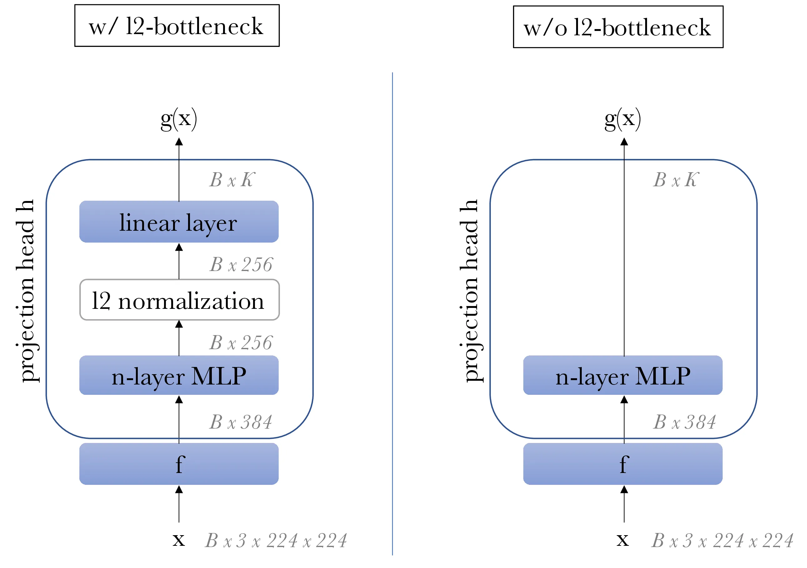
C. Projection Head
| ViT-S, 100 epochs | heads w/o BN | heads w/ BN |
|---|---|---|
| \(k\)-NN top-1 | 69.7 | 68.6 |
| # proj. head linear layers | 1 | 2 | 3 | 4 |
|---|---|---|---|---|
| w/ l2-norm bottleneck | - | 62.2 | 68.0 | 69.3 |
| w/o l2-norm bottleneck | 61.6 | 62.9 | 0.1 | 0.1 |
| \(K\) | 1024 | 4096 | 16384 | 65536 | 262144 |
|---|---|---|---|---|---|
| \(k\)-NN top-1 | 67.8 | 69.3 | 69.2 | 69.7 | 69.1 |
| ViT-S, 100 epochs | heads w/ GELU | heads w/ ReLU |
|---|---|---|
| \(k\)-NN top-1 | 69.7 | 68.9 |
D. Additional Ablations
| \(m\) | 0 | 0.9 | 0.99 | 0.999 |
|---|---|---|---|---|
| \(k\)-NN top-1 | 69.1 | 69.7 | 69.4 | 0.1 |
| \(\tau_t\) | 0 | 0.02 | 0.04 | 0.06 | 0.08 | 0.04 \(\to\) 0.07 |
|---|---|---|---|---|---|---|
| \(k\)-NN top-1 | 43.9 | 66.7 | 69.6 | 68.7 | 0.1 | 69.7 |
| DINO ViT-S | 100-ep | 300-ep | 800-ep |
|---|---|---|---|
| \(k\)-NN top-1 | 70.9 | 72.8 | 74.5 |
| ViT-S/16 weights | |
|---|---|
| Random weights | 22.0 |
| Supervised | 27.3 |
| DINO | 45.9 |
| DINO w/o multicrop | 45.1 |
| MoCo-v2 | 46.3 |
| BYOL | 47.8 |
| SwAV | 46.8 |
| # heads | dim | dim/head | # params | im/sec | \(k\)-NN |
|---|---|---|---|---|---|
| 6 | 384 | 64 | 21 | 1007 | 72.8 |
| 8 | 384 | 48 | 21 | 971 | 73.1 |
| 12 | 384 | 32 | 21 | 927 | 73.7 |
| 16 | 384 | 24 | 21 | 860 | 73.8 |
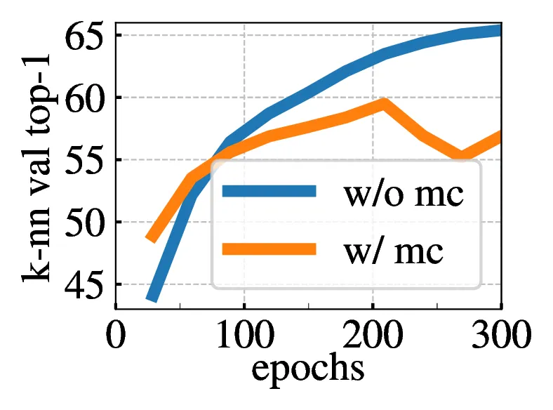
E. Multi-crop
| (0.05, s), (s, 1), s: | 0.08 | 0.16 | 0.24 | 0.32 | 0.48 |
|---|---|---|---|---|---|
| \(k\)-NN top-1 | 65.6 | 68.0 | 69.7 | 69.8 | 69.5 |
| crops | 2 × 2242 | 2 × 2242 + 6 × 962 | ||
|---|---|---|---|---|
| eval | \(k\)-NN | linear | \(k\)-NN | linear |
| BYOL | 66.6 | 71.4 | 59.8 | 64.8 |
| SwAV | 60.5 | 68.5 | 64.7 | 71.8 |
| MoCo-v2 | 62.0 | 71.6 | 65.4 | 73.4 |
| DINO | 67.9 | 72.5 | 72.7 | 75.9 |
F. Evaluation Protocols
F.1 \(k\)-NN classification
F.2 Linear classification
| concatenate \(l\) last layers | 1 | 2 | 4 | 6 |
|---|---|---|---|---|
| representation dim | 384 | 768 | 1536 | 2304 |
| ViT-S/16 linear eval | 76.1 | 76.6 | 77.0 | 77.0 |
| pooling strategy | [CLS] tok. only | concatenate [CLS] tok. and avgpooled patch tok. |
|---|---|---|
| representation dim | 768 | 1536 |
| ViT-B/16 linear eval | 78.0 | 78.2 |
G. Self-Attention Visualizations
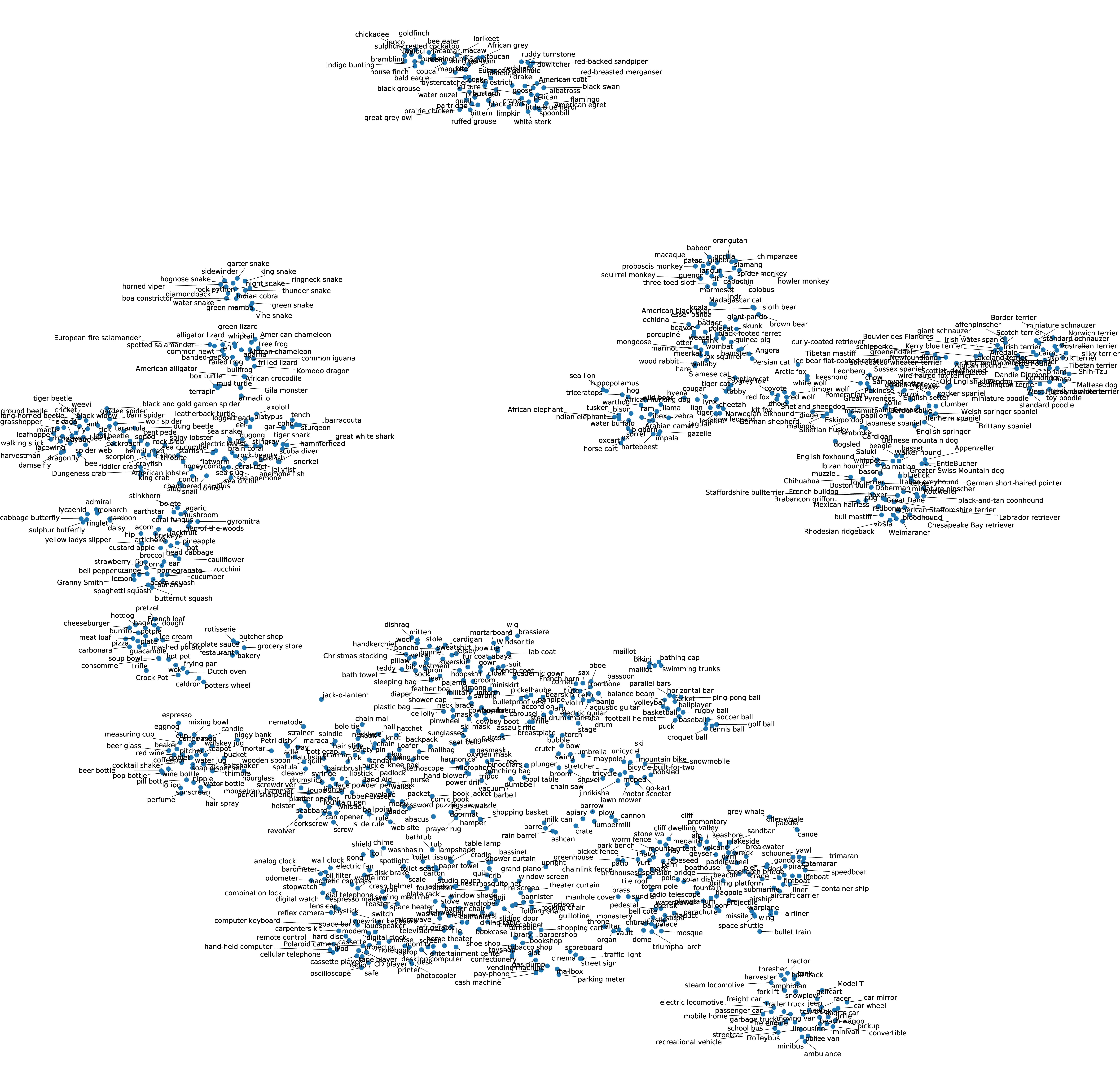
H. Class Representation
![Figure 10: Self-attention heads from the last layer. We look at the attention map when using the [CLS] token as a query for the different heads in the last layer. Note that the [CLS] token is not attached to any label or supervision.](https://img.032802.xyz/paper-reading/2021/emerging-properties-in-self-supervised-vision-transformers_2021_Caron/fig10.webp)