While the Transformer architecture has become the de-facto standard for natural language processing tasks, its applications to computer vision remain limited. In vision, attention is either applied in conjunction with convolutional networks, or used to replace certain components of convolutional networks while keeping their overall structure in place. We show that this reliance on CNNs is not necessary and a pure transformer applied directly to sequences of image patches can perform very well on image classification tasks. When pre-trained on large amounts of data and transferred to multiple mid-sized or small image recognition benchmarks (ImageNet, CIFAR-100, VTAB, etc.), Vision Transformer (ViT) attains excellent results compared to state-of-the-art convolutional networks while requiring substantially fewer computational resources to train.
An
Image is Worth 16x16 Words: Transformers for Image Recognition at
Scale
Abstract
1 Introduction
2 Related Work
3 Method
3.1 Vision Transformer (ViT)
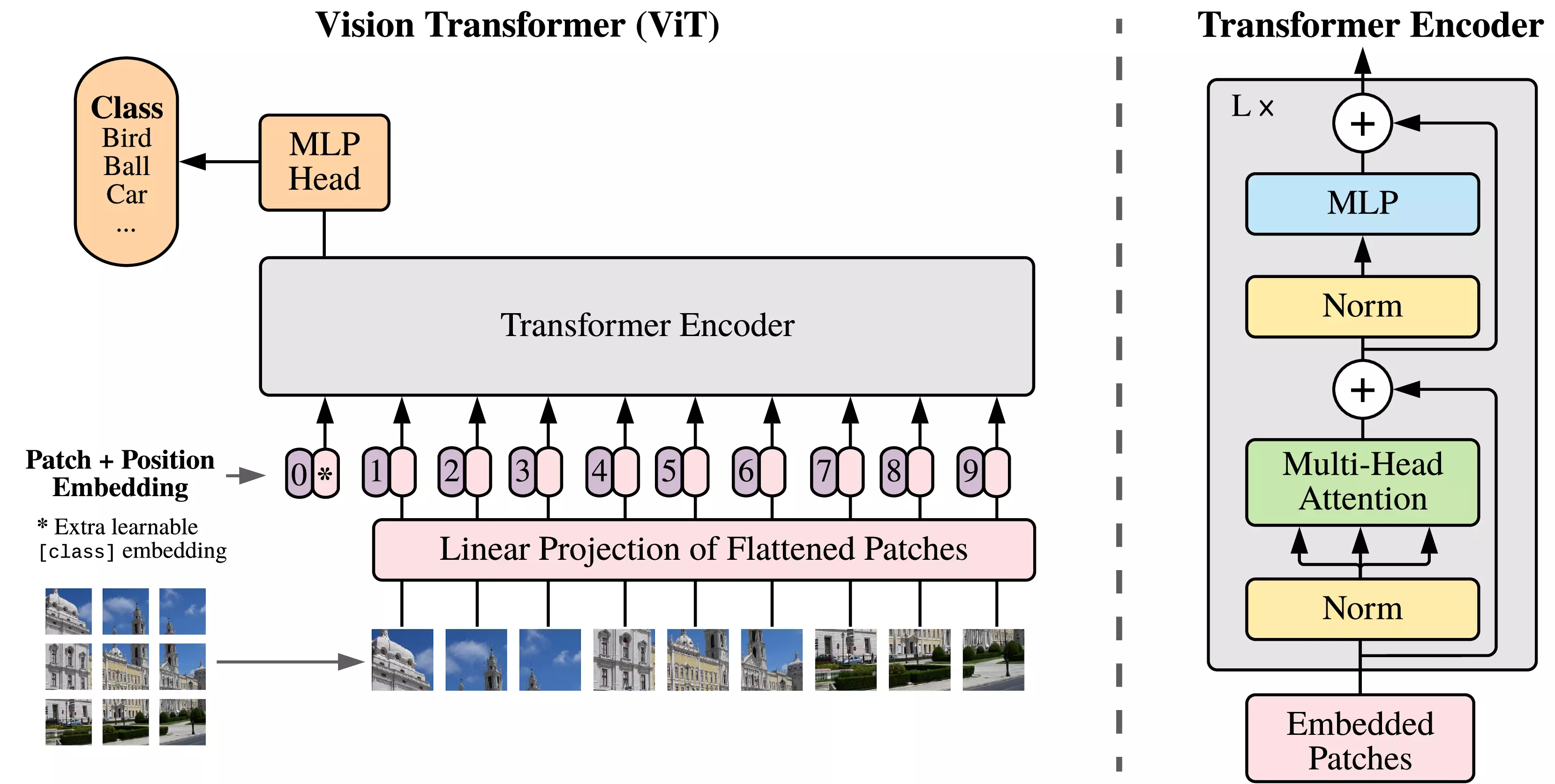
Figure 1: Model overview. We split an
image into fixed-size patches, linearly embed each of them, add position
embeddings, and feed the resulting sequence of vectors to a standard
Transformer encoder. In order to perform classification, we use the
standard approach of adding an extra learnable "classification token" to
the sequence. The illustration of the Transformer encoder was inspired
by Vaswani et al. (2017).
# Root block. x = models_resnet.StdConv( features=width, kernel_size=(7, 7), strides=(2, 2), use_bias=False, name='conv_root')(x) x = nn.GroupNorm(name='gn_root')(x) x = nn.relu(x) x = nn.max_pool(x, window_shape=(3, 3), strides=(2, 2), padding='SAME')
# ResNet stages. ifself.resnet.num_layers: x = models_resnet.ResNetStage( block_size=self.resnet.num_layers[0], nout=width, first_stride=(1, 1), name='block1')(x) for i, block_size inenumerate(self.resnet.num_layers[1:], 1): x = models_resnet.ResNetStage( block_size=block_size, nout=width * 2**i, first_stride=(2, 2), name=f'block{i + 1}')(x)
n, h, w, c = x.shape
# We can merge s2d+emb into a single conv; it's the same. x = nn.Conv( features=self.hidden_size, kernel_size=self.patches.size, strides=self.patches.size, padding='VALID', name='embedding')(x)
# Here, x is a grid of embeddings.
# (Possibly partial) Transformer. ifself.transformer isnotNone: n, h, w, c = x.shape x = jnp.reshape(x, [n, h * w, c])
# If we want to add a class token, add it here. ifself.classifier in ['token', 'token_unpooled']: cls = self.param('cls', nn.initializers.zeros, (1, 1, c)) cls = jnp.tile(cls, [n, 1, 1]) x = jnp.concatenate([cls, x], axis=1)
x = self.encoder(name='Transformer', **self.transformer)(x, train=train)
ifself.classifier == 'token': x = x[:, 0] elifself.classifier == 'gap': x = jnp.mean(x, axis=list(range(1, x.ndim - 1))) # (1,) or (1,2) elifself.classifier in ['unpooled', 'token_unpooled']: pass else: raise ValueError(f'Invalid classifier={self.classifier}')
ifself.representation_size isnotNone: x = nn.Dense(features=self.representation_size, name='pre_logits')(x) x = nn.tanh(x) else: x = IdentityLayer(name='pre_logits')(x)
ifself.num_classes: x = nn.Dense( features=self.num_classes, name='head', kernel_init=nn.initializers.zeros, bias_init=nn.initializers.constant(self.head_bias_init))(x) return x
原文:
An overview of the model is depicted in Figure 1. The standard
Transformer receives as input a 1D sequence of token embeddings. To
handle 2D images, we reshape the image \(\mathbf{x} \in \mathbb{R}^{H \times W \times
C}\) into a sequence of flattened 2D patches \(\mathbf{x}_p \in \mathbb{R}^{N \times (P^2 \cdot
C)}\), where \((H, W)\) is the
resolution of the original image, \(C\)
is the number of channels, \((P, P)\)
is the resolution of each image patch, and \(N
= \frac{H}{P} \times \frac{W}{P} = \frac{HW}{P^2}\) is the
resulting number of patches, which also serves as the effective input
sequence length for the Transformer. The Transformer uses
constant latent vector size \(D\)
through all of its layers, so we flatten the patches and map to \(D\) dimensions with a trainable linear
projection (Eq. 1). We refer to the output of this projection as the
patch embeddings.
根据原文中的说法,输入一张维度为\(\mathbf{x} \in \mathbb{R}^{H \times W \times
C}\)的图像后,ViT会将输入的形状reshape为\(\mathbf{x}_p \in \mathbb{R}^{N \times (P^2 \cdot
C)}\),其中\((H,
W)\)为原图像的分辨率,\(C\)为通道数,\((P, P)\)为每个patch的分辨率,\(N = \frac{H}{P} \times \frac{W}{P} =
\frac{HW}{P^2}\)为patch的数量,这一步没有涉及到网络操作,总的像素数\(H \times W \times C = N \times (P^2 \cdot
C)\)不变,所以直接用reshape操作即可。
后续的代码中涉及到了batch_size,为了前后统一,这里为输入图像增加一个batch_size维度,即\(\mathbf{x} \in \mathbb{R}^{n \times H \times W
\times C}\),其中\(n\)为batch_size。
classVisionTransformer(nn.Module): # ... existing code ... def__call__(self, inputs, *, train): # ... existing code ... # (Possibly partial) Transformer. ifself.transformer isnotNone: n, h, w, c = x.shape x = jnp.reshape(x, [n, h * w, c])
# If we want to add a class token, add it here. ifself.classifier in ['token', 'token_unpooled']: cls = self.param('cls', nn.initializers.zeros, (1, 1, c)) cls = jnp.tile(cls, [n, 1, 1]) x = jnp.concatenate([cls, x], axis=1)
在n, h, w, c = x.shape中,n是batch_size,h为特征图的高度\(\frac{H}{P}\),w为特征图的宽度\(\frac{W}{P}\),c为特征图的通道数\(D\),经过reshape后,batch_size不变,特征图的高度\(\frac{H}{P}\)和宽度\(\frac{W}{P}\)相乘,得到\(N\),即patch的数量,至此,reshape操作和线性映射操作结束,得到序列的维度为\(\mathbb{R}^{n \times N \times D}\)。
classEncoder(nn.Module): """Transformer Model Encoder for sequence to sequence translation. Attributes: num_layers: number of layers mlp_dim: dimension of the mlp on top of attention block num_heads: Number of heads in nn.MultiHeadDotProductAttention dropout_rate: dropout rate. attention_dropout_rate: dropout rate in self attention. """
num_layers: int mlp_dim: int num_heads: int dropout_rate: float = 0.1 attention_dropout_rate: float = 0.1 add_position_embedding: bool = True
@nn.compact def__call__(self, x, *, train): """Applies Transformer model on the inputs. Args: x: Inputs to the layer. train: Set to `True` when training. Returns: output of a transformer encoder. """ assert x.ndim == 3# (batch, len, emb)
ifself.add_position_embedding: x = AddPositionEmbs( posemb_init=nn.initializers.normal(stddev=0.02), # from BERT. name='posembed_input')(x) x = nn.Dropout(rate=self.dropout_rate)(x, deterministic=not train)
# Input Encoder for lyr inrange(self.num_layers): x = Encoder1DBlock( mlp_dim=self.mlp_dim, dropout_rate=self.dropout_rate, attention_dropout_rate=self.attention_dropout_rate, name=f'encoderblock_{lyr}', num_heads=self.num_heads)(x, deterministic=not train) encoded = nn.LayerNorm(name='encoder_norm')(x)
@nn.compact def__call__(self, inputs): """Applies the AddPositionEmbs module. Args: inputs: Inputs to the layer. Returns: Output tensor with shape `(bs, timesteps, in_dim)`. """ # inputs.shape is (batch_size, seq_len, emb_dim). assert inputs.ndim == 3, ('Number of dimensions should be 3,' ' but it is: %d' % inputs.ndim) pos_emb_shape = (1, inputs.shape[1], inputs.shape[2]) pe = self.param( 'pos_embedding', self.posemb_init, pos_emb_shape, self.param_dtype) return inputs + pe
ifself.representation_size isnotNone: x = nn.Dense(features=self.representation_size, name='pre_logits')(x) x = nn.tanh(x) else: x = IdentityLayer(name='pre_logits')(x)
ifself.num_classes: x = nn.Dense( features=self.num_classes, name='head', kernel_init=nn.initializers.zeros, bias_init=nn.initializers.constant(self.head_bias_init))(x) return x
Table 1: Details of Vision Transformer model variants.
Model
Layers
Hidden size \(D\)
MLP size
Heads
Params
ViT-Base
12
768
3072
12
86M
ViT-Large
24
1024
4096
16
307M
ViT-Huge
32
1280
5120
16
632M
Table 2: Comparison with state of the art on popular image
classification benchmarks. We report mean and standard deviation of the
accuracies, averaged over three fine-tuning runs. Vision Transformer
models pre-trained on the JFT-300M dataset outperform ResNet-based
baselines on all datasets, while taking substantially less computational
resources to pre-train. ViT pre-trained on the smaller public
ImageNet-21k dataset performs well too. ∗Slightly improved
88.5% result reported in Touvron et al. (2020).
Ours-JFT (ViT-H/14)
Ours-JFT (ViT-L/16)
Ours-i21k (ViT-L/16)
BiT-L (ResNet152x4)
Noisy Student (EfficientNet-L2)
ImageNet
88.55 ±0.04
87.76 ±0.03
85.30 ±0.02
87.54 ±0.02
88.4/88.5∗
ImageNet ReaL
90.72 ±0.05
90.54 ±0.03
88.62 ±0.05
90.54
90.55
CIFAR-10
99.50 ±0.06
99.42 ±0.03
99.15 ±0.03
99.37 ±0.06
-
CIFAR-100
94.55 ±0.04
93.90 ±0.05
93.25 ±0.05
93.51 ±0.08
-
Oxford-IIIT Pets
97.56 ±0.03
97.32 ±0.11
94.67 ±0.15
96.62 ±0.23
-
Oxford Flowers-102
99.68 ±0.02
99.74 ±0.00
99.61 ±0.02
99.63 ±0.03
-
VTAB (19 tasks)
77.63 ±0.23
76.28 ±0.46
72.72 ±0.21
76.29 ±1.70
-
TPUv3-core-days
2.5k
0.68k
0.23k
9.9k
12.3k
4.2 Comparison to State of the
Art
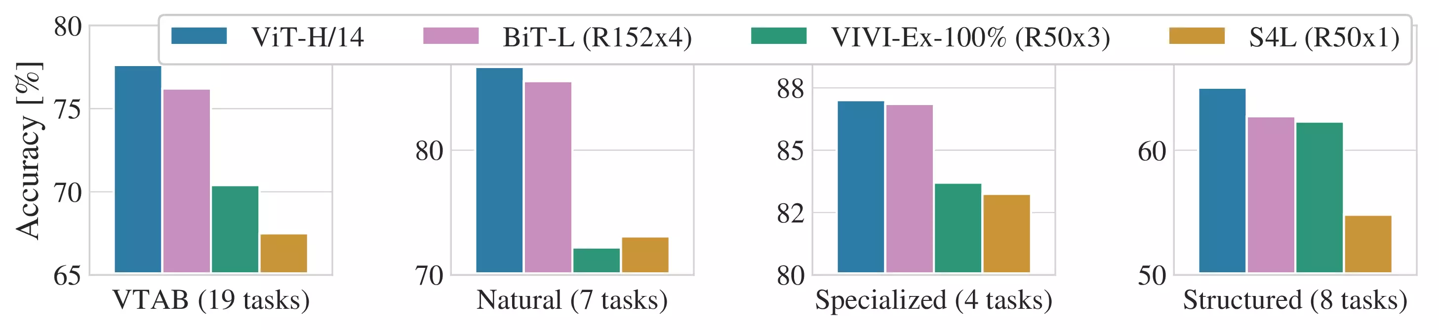
Figure 2: Breakdown of VTAB performance
in Natural, Specialized, and Structured task groups.
4.3 Pre-training Data
Requirements
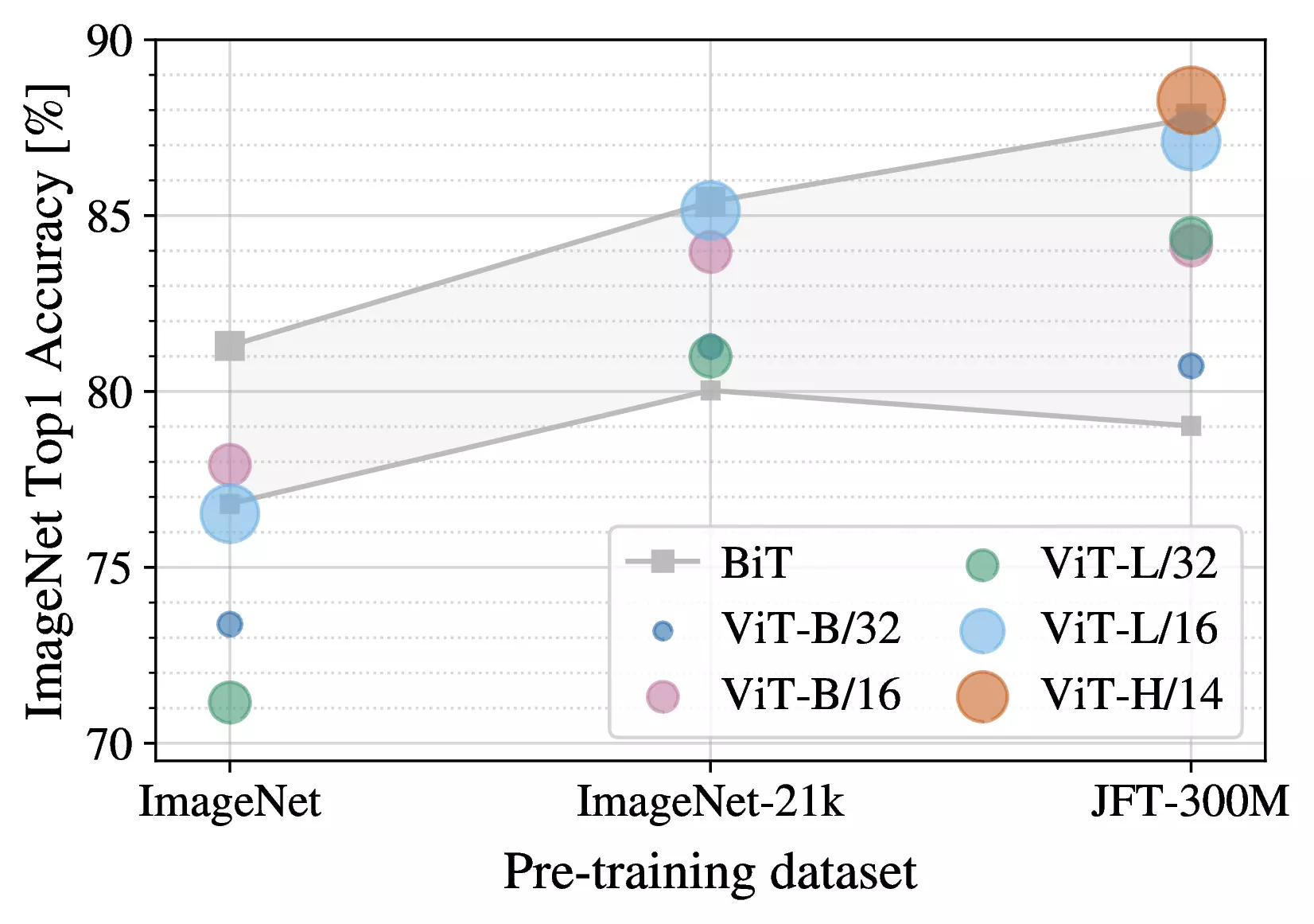
Figure 3: Transfer to ImageNet. While
large ViT models perform worse than BiT ResNets (shaded area) when
pre-trained on small datasets, they shine when pre-trained on larger
datasets. Similarly, larger ViT variants overtake smaller ones as the
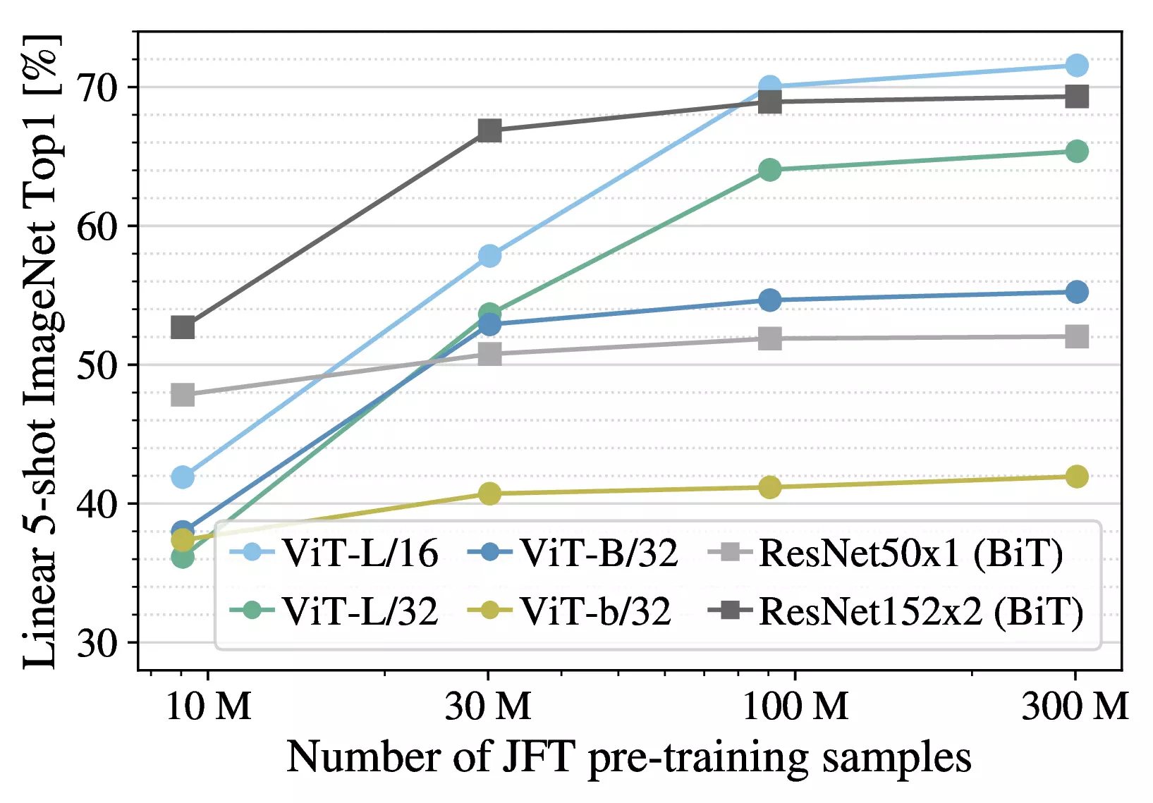
dataset grows.Figure 4: Linear few-shot evaluation on
ImageNet versus pre-training size. ResNets perform better with smaller
pre-training datasets but plateau sooner than ViT, which performs better
with larger pre-training. ViT-b is ViT-B with all hidden dimensions
halved.
Table 5: Top1 accuracy (in %) of Vision Transformer on various datasets
when pre-trained on ImageNet, ImageNet-21k or JFT300M. These values
correspond to Figure 3 in the main text. Models are fine-tuned at 384
resolution. Note that the ImageNet results are computed without
additional techniques (Polyak averaging and 512 resolution images) used
to achieve results in Table 2.
ViT-B/16
ViT-B/32
ViT-L/16
ViT-L/32
ViT-H/14
ImageNet
CIFAR-10
98.13
97.77
97.86
97.94
-
CIFAR-100
87.13
86.31
86.35
87.07
-
ImageNet
77.91
73.38
76.53
71.16
-
ImageNet ReaL
83.57
79.56
82.19
77.83
-
Oxford Flowers-102
89.49
85.43
89.66
86.36
-
Oxford-IIIT-Pets
93.81
92.04
93.64
91.35
-
ImageNet-21k
CIFAR-10
98.95
98.79
99.16
99.13
99.27
CIFAR-100
91.67
91.97
93.44
93.04
93.82
ImageNet
83.97
81.28
85.15
80.99
85.13
ImageNet ReaL
88.35
86.63
88.40
85.65
88.70
Oxford Flowers-102
99.38
99.11
99.61
99.19
99.51
Oxford-IIIT-Pets
94.43
93.02
94.73
93.09
94.82
JFT-300M
CIFAR-10
99.00
98.61
99.38
99.19
99.50
CIFAR-100
91.87
90.49
94.04
92.52
94.55
ImageNet
84.15
80.73
87.12
84.37
88.04
ImageNet ReaL
88.85
86.27
89.99
88.28
90.33
Oxford Flowers-102
99.56
99.27
99.56
99.45
99.68
Oxford-IIIT-Pets
95.80
93.40
97.11
95.83
97.56
4.4 Scaling Study
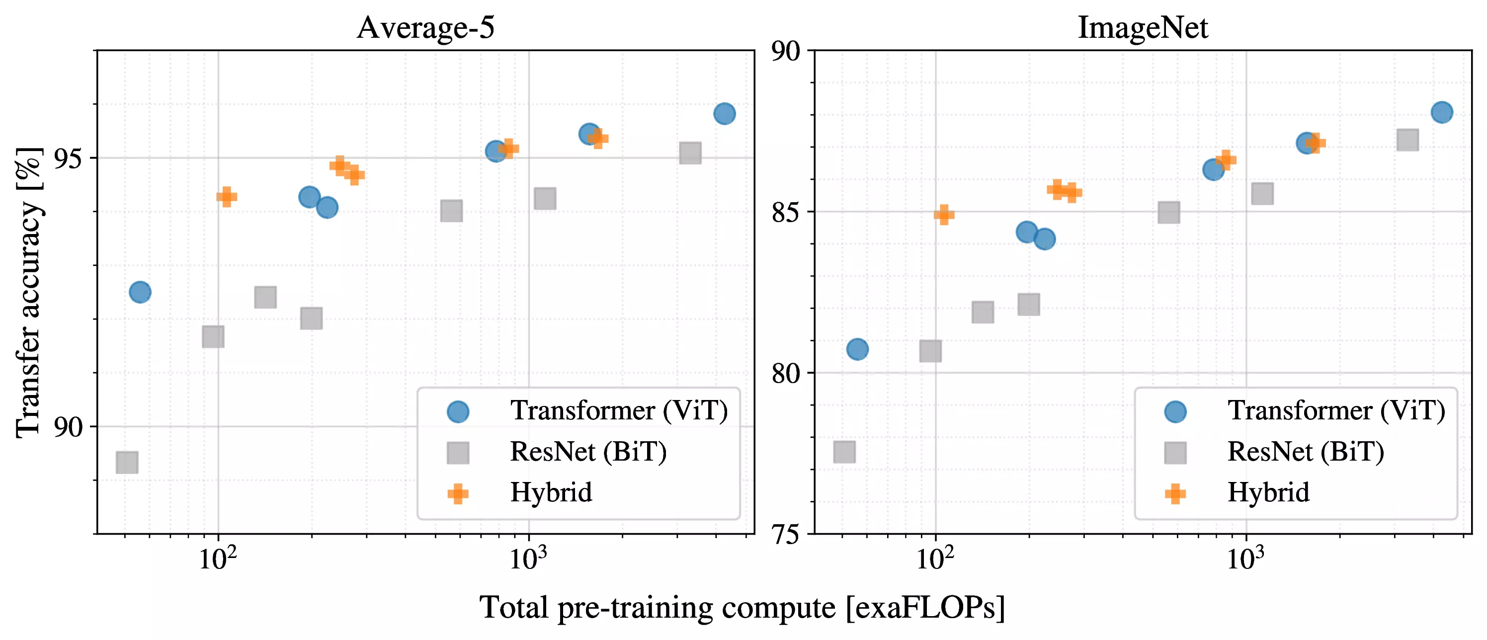
Figure 5: Performance versus pre-training
compute for different architectures: Vision Transformers, ResNets, and
hybrids. Vision Transformers generally outperform ResNets with the same
computational budget. Hybrids improve upon pure Transformers for smaller
model sizes, but the gap vanishes for larger models.
Table 6: Detailed results of model scaling experiments. These correspond
to Figure 5 in the main paper. We show transfer accuracy on several
datasets, as well as the pre-training compute (in exaFLOPs).
name
Epochs
ImageNet
ImageNet ReaL
CIFAR-10
CIFAR-100
Pets
Flowers
exaFLOPs
ViT-B/32
7
80.73
86.27
98.61
90.49
93.40
99.27
55
ViT-B/16
7
84.15
88.85
99.00
91.87
95.80
99.56
224
ViT-L/32
7
84.37
88.28
99.19
92.52
95.83
99.45
196
ViT-L/16
7
86.30
89.43
99.38
93.46
96.81
99.66
783
ViT-L/16
14
87.12
89.99
99.38
94.04
97.11
99.56
1567
ViT-H/14
14
88.08
90.36
99.50
94.71
97.11
99.71
4262
ResNet50x1
7
77.54
84.56
97.67
86.07
91.11
94.26
50
ResNet50x2
7
82.12
87.94
98.29
89.20
93.43
97.02
199
ResNet101x1
7
80.67
87.07
98.48
89.17
94.08
95.95
96
ResNet152x1
7
81.88
87.96
98.82
90.22
94.17
96.94
141
ResNet152x2
7
84.97
89.69
99.06
92.05
95.37
98.62
563
ResNet152x2
14
85.56
89.89
99.24
91.92
95.75
98.75
1126
ResNet200x3
14
87.22
90.15
99.34
93.53
96.32
99.04
3306
R50x1+ViT-B/32
7
84.90
89.15
99.01
92.24
95.75
99.46
106
R50x1+ViT-B/16
7
85.58
89.65
99.14
92.63
96.65
99.40
274
R50x1+ViT-L/32
7
85.68
89.04
99.24
92.93
96.97
99.43
246
R50x1+ViT-L/16
7
86.60
89.72
99.18
93.64
97.03
99.40
859
R50x1+ViT-L/16
14
87.12
89.76
99.31
93.89
97.36
99.11
1668
4.5 Inspecting Vision
Transformer
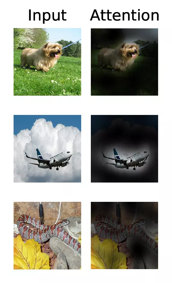
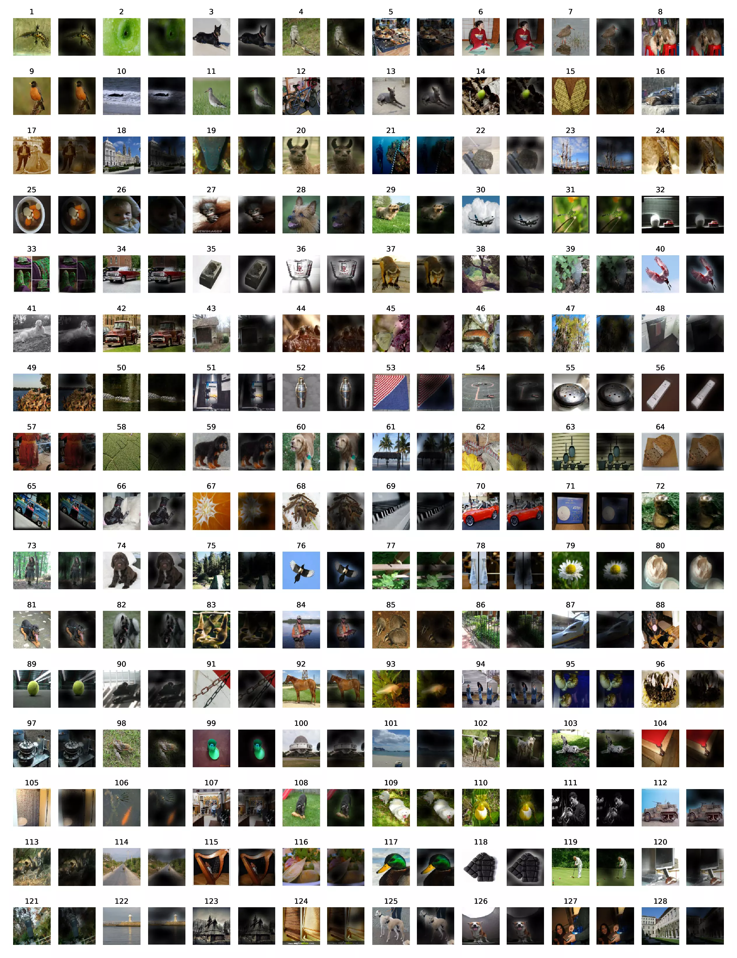
Figure 6: Representative examples of
attention from the output token to the input space. See Appendix D.7 for
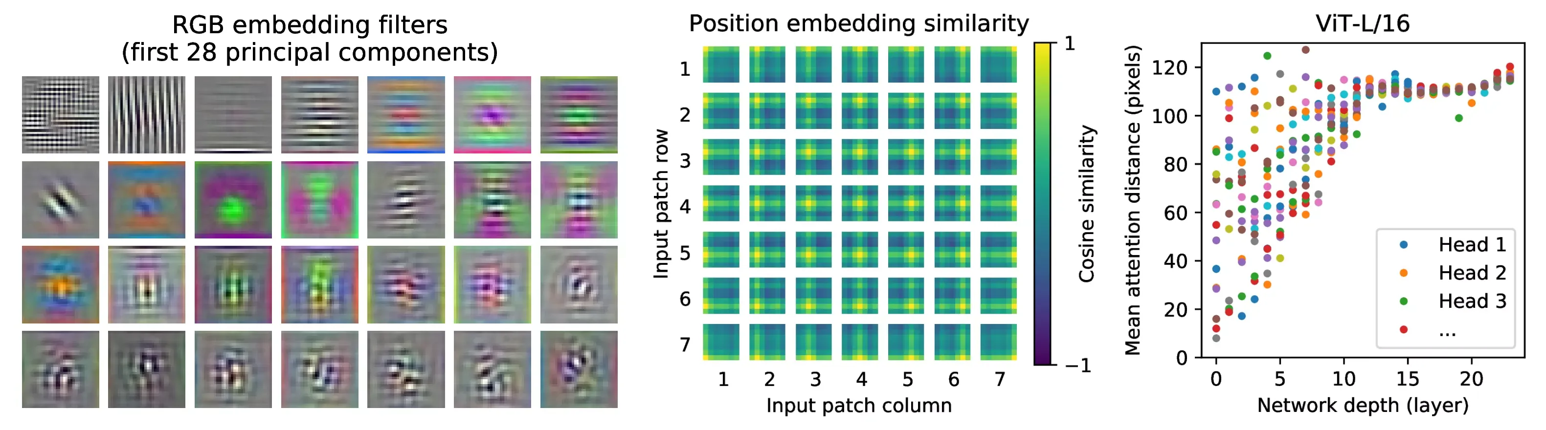
details.Figure 7: Left: Filters of the initial
linear embedding of RGB values of ViT-L/32. Center: Similarity of
position embeddings of ViT-L/32. Tiles show the cosine similarity
between the position embedding of the patch with the indicated row and
column and the position embeddings of all other patches. Right: Size of
attended area by head and network depth. Each dot shows the mean
attention distance across images for one of 16 heads at one layer. See
Appendix D.7 for details.
4.6 Self-supervision
5 Conclusion
Appendix
A Multihead Self-attention
B Experiment Details
B.1 Training
Table 3: Hyperparameters for training. All models are trained with a
batch size of 4096 and learning rate warmup of 10k steps. For ImageNet
we found it beneficial to additionally apply gradient clipping at global
norm 1. Training resolution is 224.
Models
Dataset
Epochs
Base LR
LR decay
Weight decay
Dropout
ViT-B/{16,32}
JFT-300M
7
8 · 10-4
linear
0.1
0.0
ViT-L/32
JFT-300M
7
6 · 10-4
linear
0.1
0.0
ViT-L/16
JFT-300M
7/14
4 · 10-4
linear
0.1
0.0
ViT-H/14
JFT-300M
14
3 · 10-4
linear
0.1
0.0
R50x{1,2}
JFT-300M
7
10-3
linear
0.1
0.0
R101x1
JFT-300M
7
8 · 10-4
linear
0.1
0.0
R152x{1,2}
JFT-300M
7
6 · 10-4
linear
0.1
0.0
R50+ViT-B/{16,32}
JFT-300M
7
8 · 10-4
linear
0.1
0.0
R50+ViT-L/32
JFT-300M
7
2 · 10-4
linear
0.1
0.0
R50+ViT-L/16
JFT-300M
7/14
4 · 10-4
linear
0.1
0.0
ViT-B/{16,32}
ImageNet-21k
90
10-3
linear
0.03
0.1
ViT-L/{16,32}
ImageNet-21k
30/90
10-3
linear
0.03
0.1
ViT-∗
ImageNet
300
3 · 10-3
cosine
0.3
0.1
B.1.1 Fine-tuning
Table 4: Hyperparameters for fine-tuning. All models are fine-tuned with
cosine learning rate decay, a batch size of 512, no weight decay, and
grad clipping at global norm 1. If not mentioned otherwise, fine-tuning
resolution is 384.
Dataset
Steps
Base LR
ImageNet
20000
{0.003, 0.01, 0.03, 0.06}
CIFAR100
10000
{0.001, 0.003, 0.01, 0.03}
CIFAR10
10000
{0.001, 0.003, 0.01, 0.03}
Oxford-IIIT Pets
500
{0.001, 0.003, 0.01, 0.03}
Oxford Flowers-102
500
{0.001, 0.003, 0.01, 0.03}
VTAB (19 tasks)
2500
0.01
B.1.2 Self-supervision
C Additional Results
D Additional Analyses
D.1 Sgd Vs. Adam For Resnets
Table 7: Fine-tuning ResNet models pre-trained with Adam and SGD.
Dataset
ResNet50
ResNet152x2
Adam
SGD
Adam
SGD
ImageNet
77.54
78.24
84.97
84.37
CIFAR10
97.67
97.46
99.06
99.07
CIFAR100
86.07
85.17
92.05
91.06
Oxford-IIIT Pets
91.11
91.00
95.37
94.79
Oxford Flowers-102
94.26
92.06
98.62
99.32
Average
89.33
88.79
94.01
93.72
D.2 Transformer Shape
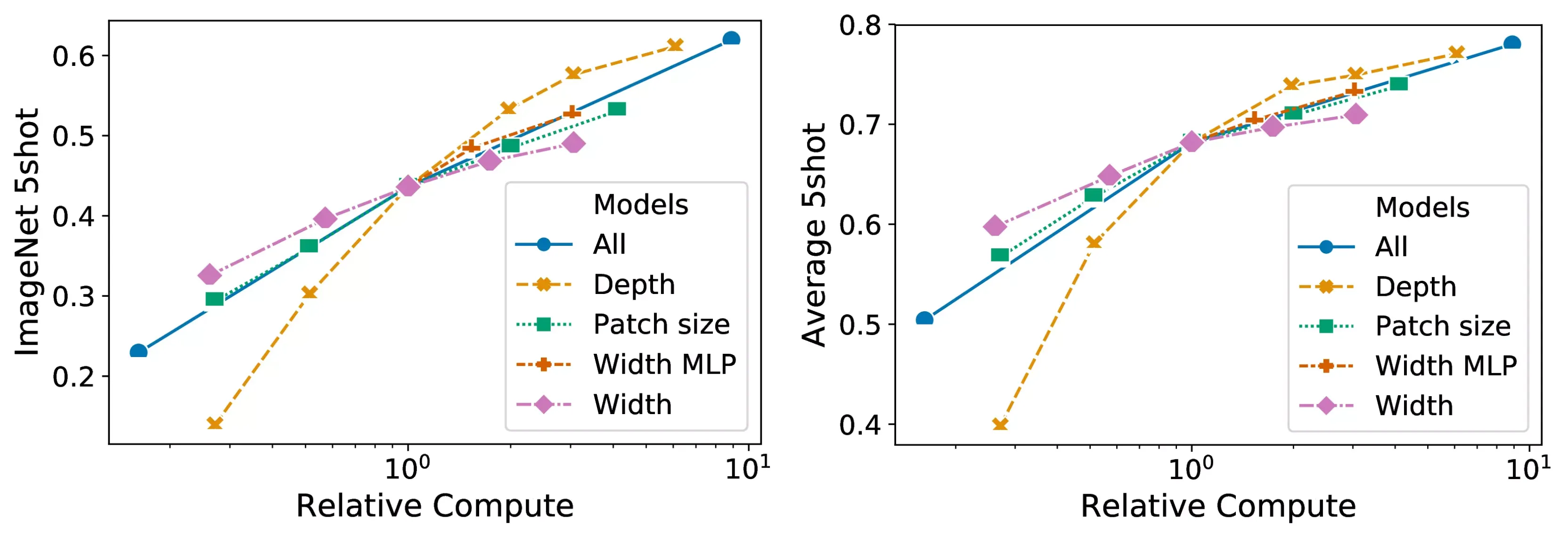
Figure 8: Scaling different model
dimensions of the Vision Transformer.
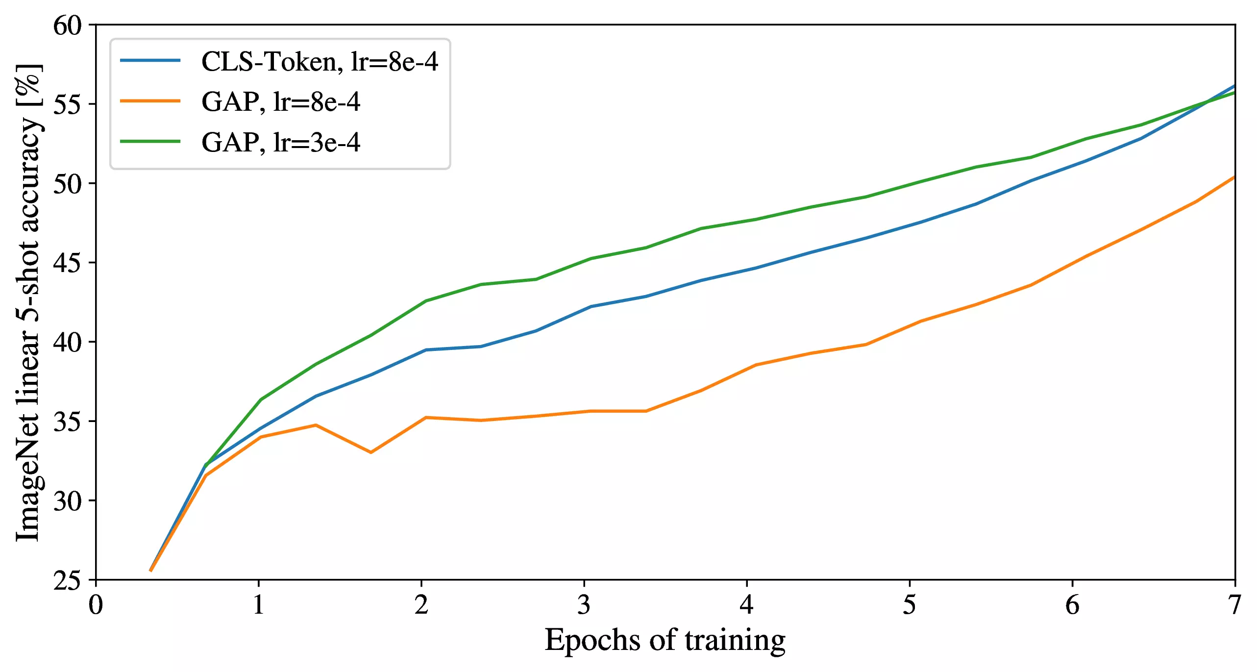
D.3 Head Type And Class
Token
Figure 9: Comparison of class-token and
global average pooling classifiers. Both work similarly well, but
require different learning-rates.
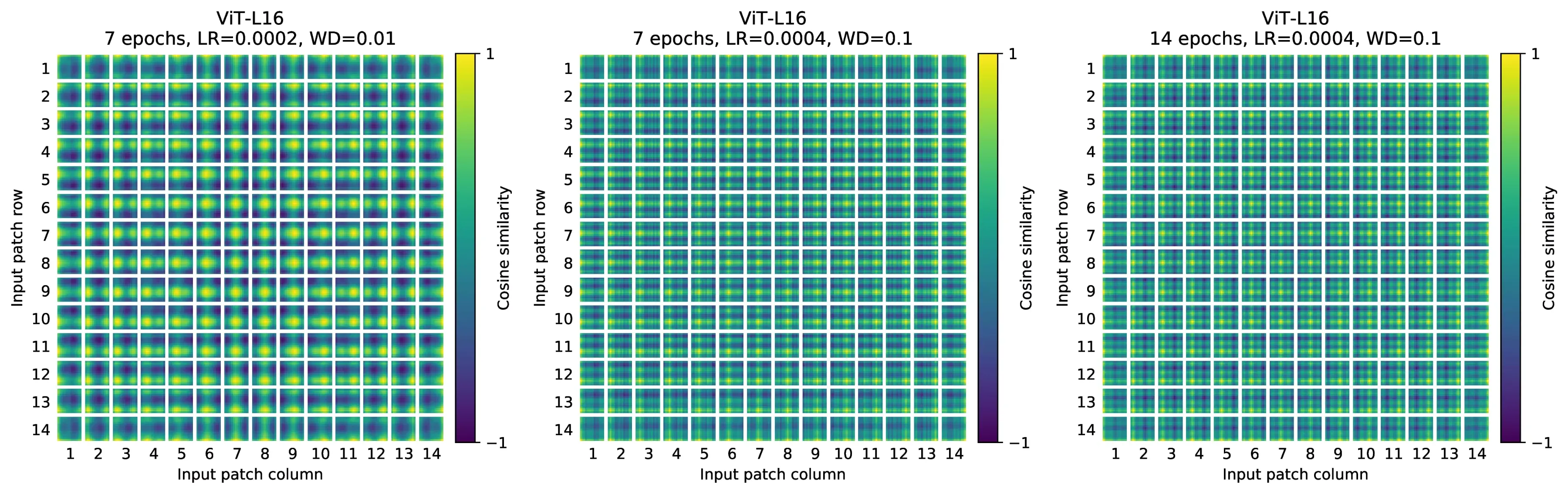
D.4 Positional Embedding
Figure 10: Position embeddings of models
trained with different hyperparameters.
Table 8: Results of the ablation study on positional embeddings with
ViT-B/16 model evaluated on ImageNet 5-shot linear.
Pos. Emb.
Default/Stem
Every Layer
Every Layer-Shared
No Pos. Emb.
0.61382
N/A
N/A
1-D Pos. Emb.
0.64206
0.63964
0.64292
2-D Pos. Emb.
0.64001
0.64046
0.64022
Rel. Pos. Emb.
0.64032
N/A
N/A
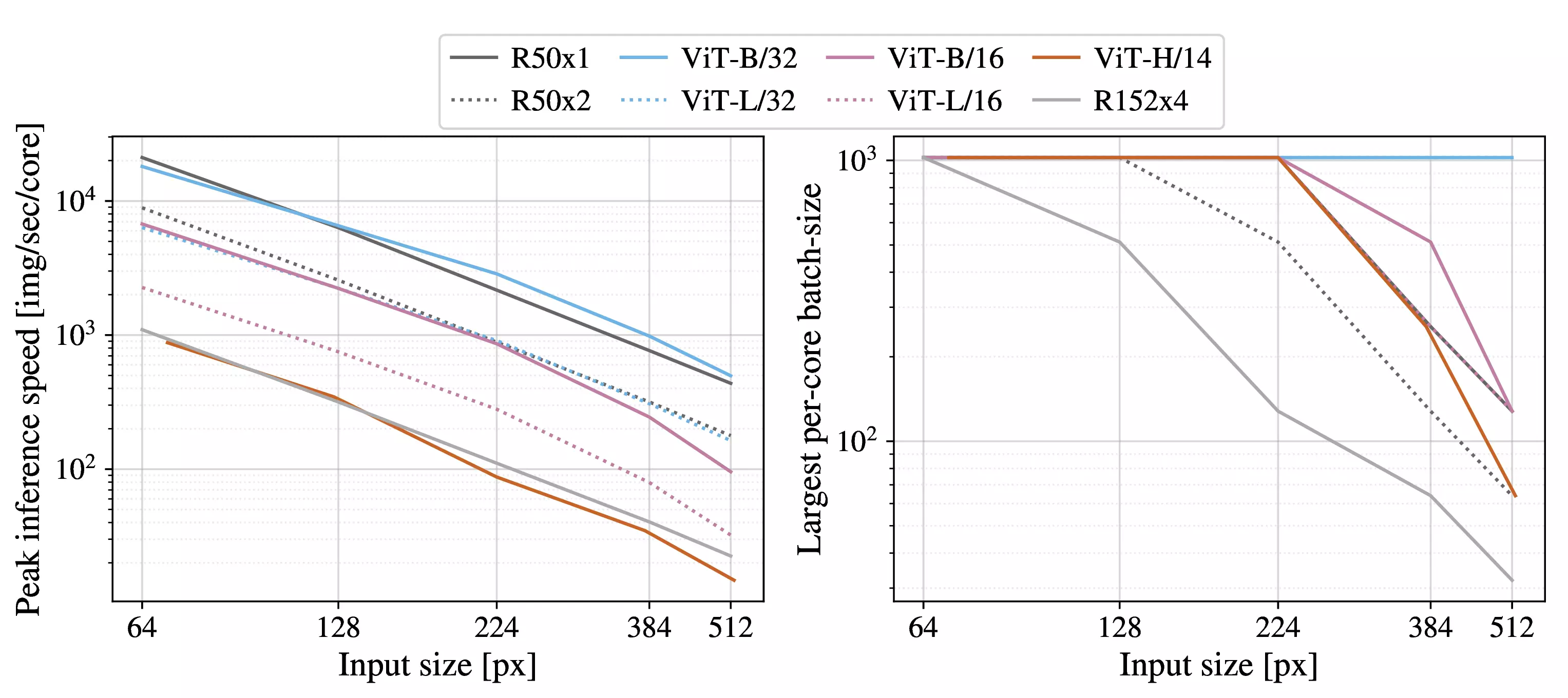
D.5 Empirical Computational
Costs
Figure 12: Left: Real wall-clock timings
of various architectures across input sizes. ViT models have speed
comparable to similar ResNets. Right: Largest per-core batch-size
fitting on device with various architectures across input sizes. ViT
models are clearly more memory-efficient.
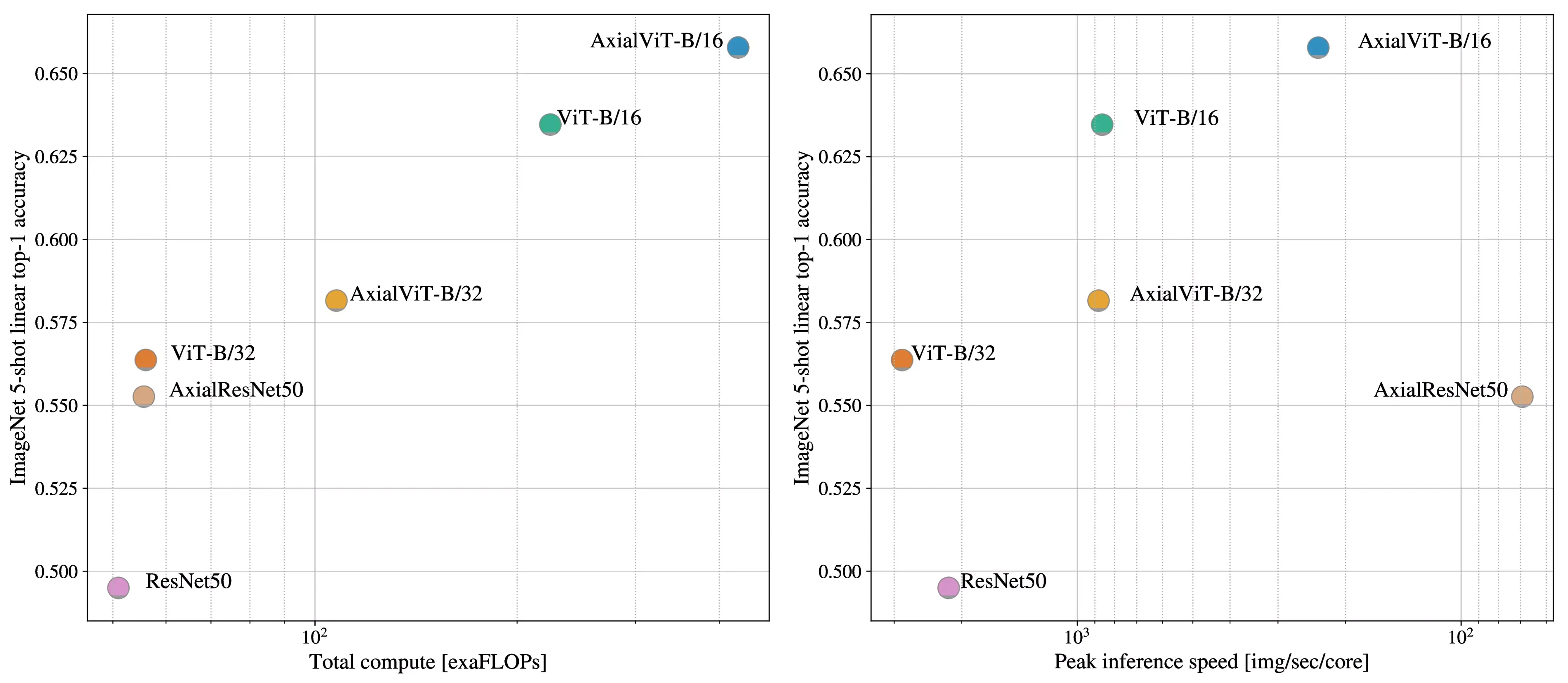
D.6 Axial Attention
Figure 13: Performance of Axial-Attention
based models, in terms of top-1 accuracy on ImageNet 5-shot linear,
versus their speed in terms of number of FLOPs.
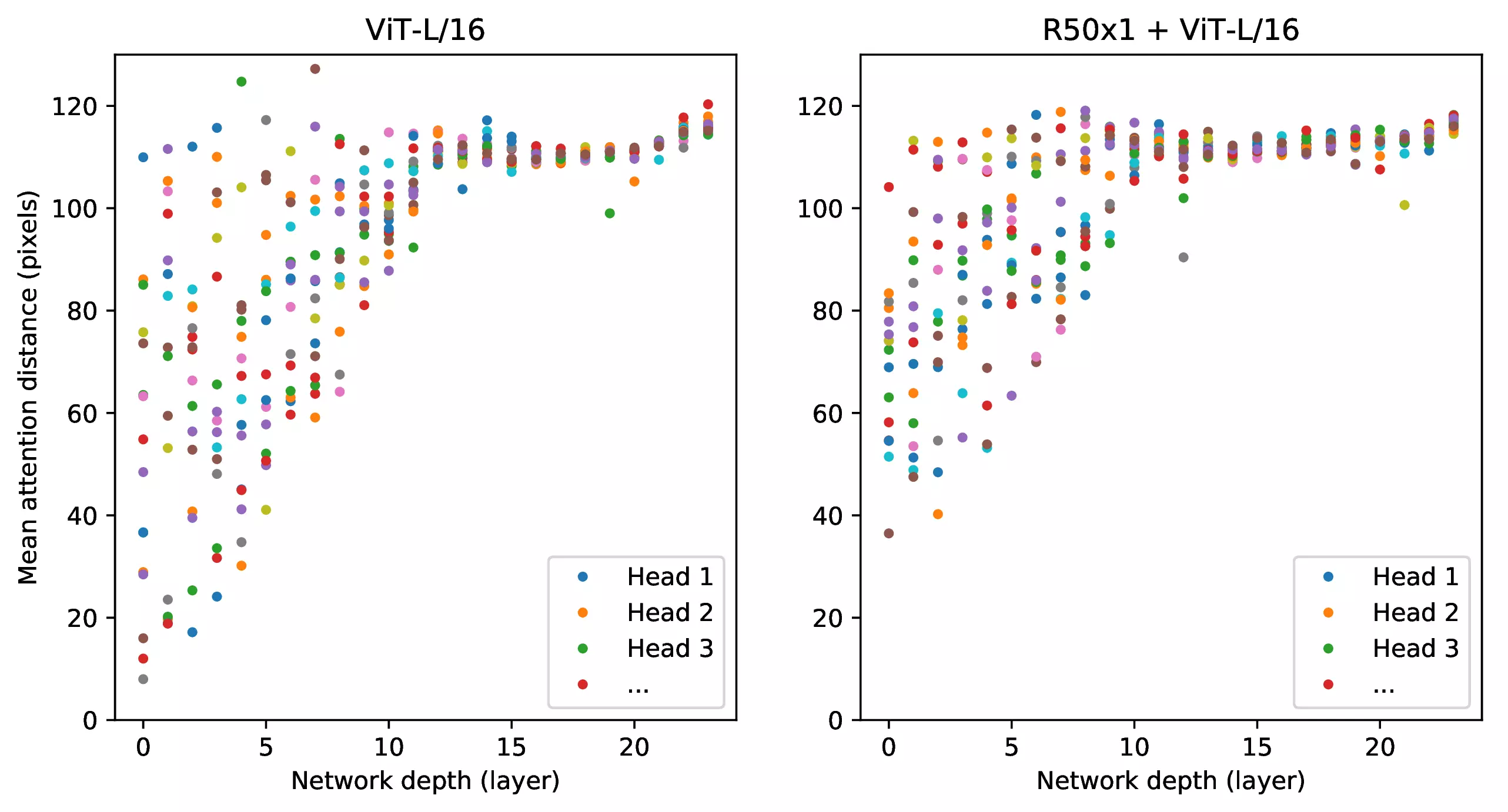
D.7 Attention Distance
Figure 11: Size of attended area by head
and network depth. Attention distance was computed for 128 example
images by averaging the distance between the query pixel and all other
pixels, weighted by the attention weight. Each dot shows the mean
attention distance across images for one of 16 heads at one layer. Image
width is 224 pixels.
D.8 Attention Maps
D.9 Objectnet Results
D.10 VTAB Breakdown
Figure 14: Further example attention maps
as in Figure 6 (random selection).
Table 9: Breakdown of VTAB-1k performance across tasks.