【论文笔记】6D-Diff: A Keypoint Diffusion Framework for 6D Object Pose Estimation
6D-Diff: A Keypoint Diffusion Framework for 6D Object Pose Estimation
| 方法 | 类型 | 训练输入 | 推理输入 | 输出 | pipeline |
|---|---|---|---|---|---|
| 6D-Diff | 实例级 | RGB + CAD | RGB + CAD(应该是需要CAD的) | 绝对\(\mathbf{R}, \mathbf{t}\) |
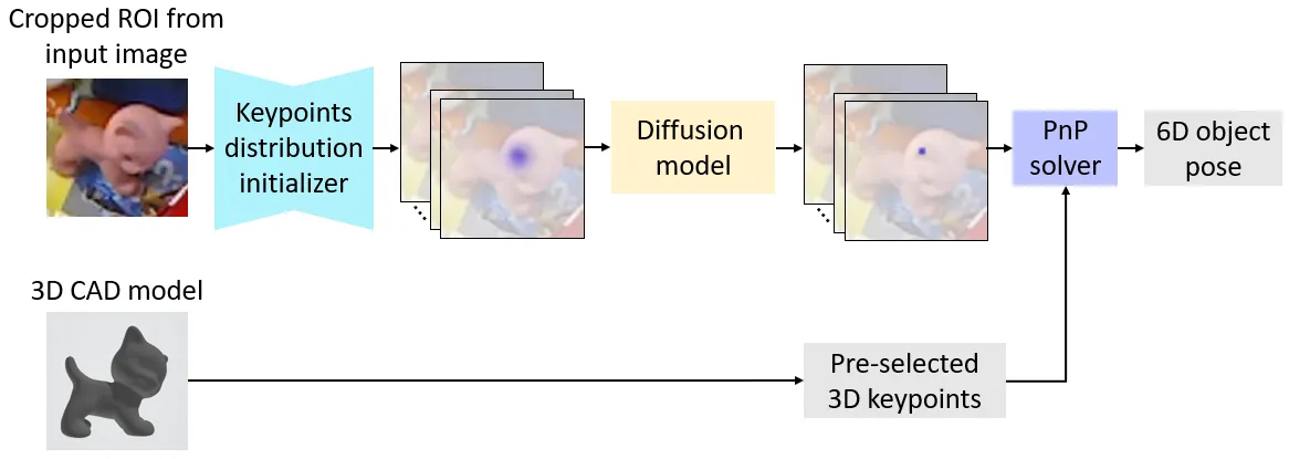
- 2025.02.26:代码未开源,方法倒是看懂了,从扩散模型中获得灵感,学习一个去除关键点噪声的反向过程,得到2D-3D对应关系,然后使用PnP求解位姿
Abstract
1. Introduction
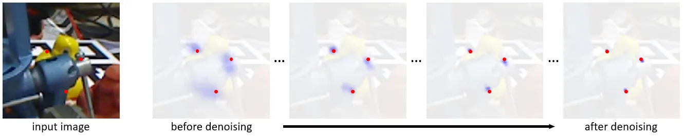
![Figure 2. Above we show two examples of keypoint heatmaps, which serve as the intermediate representation [4, 5, 44] in our framework. The red dots indicate the ground-truth locations of the keypoints. In the example (a), the target object is the pink cat, which is heavily occluded in the image and is shown in a different pose compared to the 3D model. As shown above, due to occlusions and cluttered backgrounds, the keypoint heatmaps are noisy, which reflects the noise and indeterminacy during the keypoints detection process.](https://img.032802.xyz/paper-reading/2024/6d-diff-a-keypoint-diffusion-framework-for-6d-object-pose-estimation_2024_Xu/fig_demo.webp)
Our work makes the following contributions:
- We propose a novel 6D-Diff framework, in which we formulate keypoints detection for 6D object pose estimation as a reverse diffusion process to effectively eliminate the noise and indeterminacy in object pose estimation.
- To take advantage of the intermediate representation that encodes useful prior distribution knowledge for handling this task, we propose a novel MoC-based diffusion process.
- Besides, we facilitate the model learning by utilizing object features.
2. Related Work
3. Method
总结:
训练:
- 给定RGB和物体CAD,先使用已有的目标检测将ROI框出来,然后在CAD上使用FPS选3D点(方法中选了\(N = 128\)个),由于GT Pose已知,所以可以将3D点投影到图像2D点上,得到2D点的坐标;
- 使用这些2D点,基于“Making Deep Heatmaps Robust to Partial Occlusions for 3D Object Pose Estimation”的方法生成热图(\(N = 128\)个),同时得到外观特征\(f_\text{app}\);
- 将得到的热图转换为概率分布\(D_K\)(只有一个),然后使用EM算法将其描述为柯西混合(MoC)分布\(\hat{D}_K\);
- 由于有真实的2D关键点坐标\(d_0 \in \mathbb{R}^{N \times 2}\),我们可以从柯西混合分布\(\hat{D}_K\)中基于\(\hat{d}_k = \sqrt{\bar{\alpha}_k}d_0 + (1 - \sqrt{\bar{\alpha}_k})\mu^{\text{MoC}} + \sqrt{1 - \bar{\alpha}_k}\epsilon^\text{MoC}\)采样噪声得到\(\{\hat{d}_1, \cdots, \hat{d}_K\}\),我们采样\(M = 5\)次,可以得到\(M\)组\(\{\hat{d}_1, \cdots, \hat{d}_K\}\),即\(\{\hat{d}_1^i, \cdots, \hat{d}_K^i\}_{i = 1}^M\);
- 然后基于这\(M = 5\)组数据,迭代去噪,得到\(M = 5\)个结果,取平均,得到2D-3D对应关系,使用PnP求解位姿;
测试:
- 给定RGB,生成热图,初始化\(D_K\),转换到\(\hat{D}_K\);
- 从\(\hat{D}_K\)中采样\(M = 5\)组\(d_K\),得到\(\{\hat{d}_K^i\}_{i = 1}^M\);
- 使用反向过程去噪,得到\(\{\hat{d}_0^i\}_{i = 1}^M\);
- 取平均,得到2D-3D对应关系,使用PnP求解位姿。
3.1. Revisiting Diffusion Models
扩散模型是一种概率生成模型,它由两个部分组成,即正向过程和反向过程。具体来说,给定一个原始样本\(d_0\)(例如,一张干净的图像),将样本\(d_0\)朝着噪声(通常是高斯噪声)\(d_K \sim \mathcal{N}(\mathbf{0}, \mathbf{I})\)进行迭代扩散的过程(即\(d_0 \to d_1 \to \cdots \to d_K\))被称为正向过程。相反,将噪声\(d_K\)朝着样本\(d_0\)进行迭代去噪的过程(即\(d_K \to d_{K - 1} \to \cdots \to d_0\))被称为反向过程。每个过程都被定义为一个马尔可夫链。
Forward Process
为了获取用于训练扩散模型的监督信号,以便模型能够逐步学习执行反向过程,我们需要获取中间步骤结果\(\{d_k\}_{k = 1}^{K - 1}\)。因此,首先要执行正向过程,以生成这些用于训练的中间步骤结果。具体而言,从\(d_1\)到\(d_K\)的后验分布\(q(d_{1 : K} | d_0)\)可表示为:
\[ \begin{equation}\label{eq1} \begin{aligned} q(d_{1 : K} | d_0) &= \prod_{k = 1}^K q(d_k | d_{k - 1}) \\ q(d_k | d_{k - 1}) &= \mathcal{N}(d_k; \sqrt{1 - \beta_k}d_{k - 1}, \beta_k\mathbf{I}) \end{aligned} \end{equation} \]
其中,\(\{\beta_k \in (0, 1)\}_{k = 1}^{K}\)表示一组固定的方差控制器,它们控制着在不同步骤中注入噪声的规模。根据公式\(\eqref{eq1}\),我们可以推导出\(q(d_k | d_0)\)的闭式形式如下:
\[ \begin{equation}\label{eq2} q(d_k | d_0) = \mathcal{N}(d_k; \sqrt{\bar{\alpha}_k}d_0, (1 - \bar{\alpha}_k)\mathbf{I}) \end{equation} \]
其中,\(\alpha_k = 1 - \beta_k\),\(\bar{\alpha}_k = \prod_{s = 1}^k \alpha_s\)。根据公式\(\eqref{eq2}\),\(d_k\)可以表示为:
\[ \begin{equation}\label{eq3} d_k = \sqrt{\bar{\alpha}_k}d_0 + \sqrt{1 - \bar{\alpha}_k}\epsilon \end{equation} \]
其中,\(\epsilon \sim \mathcal{N}(\mathbf{0}, \mathbf{I})\)。
公式\(\eqref{eq3}\)的推导过程如下:
当\(k = 1\)时,有\(q(d_1 | d_0) = \mathcal{N}(d_1; \sqrt{1 - \beta_1}d_0, \beta_1\mathbf{I})\),根据正态分布的性质,如果\(X \sim \mathcal{N}(\mu, \sigma^2)\),那么我们可以将\(X\)表示为:\(X = \mu + \sigma\epsilon\),其中\(\epsilon \sim \mathcal{N}(0, 1)\),那么有:
\[ d_1 = \sqrt{1 - \beta_1}d_0 + \sqrt{\beta_1}\epsilon_1, \]
当\(k = 2\)时,有:
\[ d_2 = \sqrt{1 - \beta_2}d_1 + \sqrt{\beta_2}\epsilon_2, \]
将\(d_1\)代入\(d_2\),有:
\[ \begin{aligned} d_2 &= \sqrt{1 - \beta_2}\left(\sqrt{1 - \beta_1}d_0 + \sqrt{\beta_1}\epsilon_1\right) + \sqrt{\beta_2}\epsilon_2, \\ d_2 &= \sqrt{(1 - \beta_1)(1 - \beta_2)}d_0 + \sqrt{\beta_1(1 - \beta_2)}\epsilon_1 + \sqrt{\beta_2}\epsilon_2, \end{aligned} \]
注意,对于两个正态分布\(X \sim \mathcal{N}(\mu_1, \sigma_1^2)\)和\(Y \sim \mathcal{N}(\mu_2, \sigma_2^2)\),如果它们独立,那么这两个正态分布的线性组合仍然是正态分布,即\(aX + bY \sim \mathcal{N}(a\mu_1 + b\mu_2, a^2\sigma_1^2 + b^2\sigma_2^2)\)(也可写为\(aX + bY \sim (a\mu_1 + b\mu_2) + \sqrt{a^2\sigma_1^2 + b^2\sigma_2^2}\epsilon\)),由于\(\epsilon_1, \epsilon_2 \sim \mathcal{N}(0, 1)\),所以简化\(d_2\)得到:
\[ d_2 = \sqrt{(1 - \beta_1)(1 - \beta_2)}d_0 + \sqrt{\beta_1(1 - \beta_2) + \beta_2}\epsilon, \]
令\(\alpha_k = 1 - \beta_k\),有:
\[ d_2 = \sqrt{\alpha_1\alpha_2}d_0 + \sqrt{1 - \alpha_1\alpha_2}\epsilon, \]
令\(\bar{\alpha}_k = \prod_{s = 1}^k \alpha_s\),根据数学归纳法,有:
\[ d_k = \sqrt{\bar{\alpha}_k}d_0 + \sqrt{1 - \bar{\alpha}_k}\epsilon, \]
推导结束。
根据公式\(\eqref{eq3}\),我们可以观察到,当扩散步骤的数量\(K\)足够大且\(\bar{\alpha}_K\)相应地减小到几乎为零时,\(d_K\)的分布近似为标准高斯分布,即\(d_K \sim \mathcal{N}(\mathbf{0}, \mathbf{I})\)。这意味着\(d_0\)逐渐被破坏成高斯噪声,这符合扩散过程的非平衡热力学现象。
Reverse Process
借助在正向过程中获取的中间步骤结果\(\{d_k\}_{k = 1}^{K - 1}\),对扩散模型进行训练,使其学习执行反向过程。具体而言,在反向过程中,每一步都可以表示为一个函数\(f\),该函数将\(d_k\)和扩散模型\(M_\text{diff}\)作为输入,并生成\(d_{k - 1}\)作为输出,即\(d_{k - 1} = f(d_k, M_\text{diff})\)。
在训练完扩散模型之后,在推理阶段,我们无需执行正向过程。相反,我们仅执行反向过程,该过程使用经过训练的扩散模型将一个随机高斯噪声\(d_K \sim \mathcal{N}(\mathbf{0}, \mathbf{I})\)转换为所需分布的样本\(d_0\)。
3.2. Proposed Framework
与先前的研究类似,我们的框架通过两阶段的流程来预测物体的6D位姿。具体来说:
- 我们首先在物体的CAD模型上选择\(N\)个3D关键点,并在图像中检测相应的\(N\)个2D关键点;
- 然后我们使用PnP求解器来计算6D位姿。在这里,我们主要关注第一阶段,目标是得出更精确的关键点检测结果。
在检测2D关键点时,诸如遮挡和杂乱背景等因素会给这一过程带来噪声和不确定性,并影响检测结果的准确性。为了解决这个问题,受到扩散模型能够通过迭代减少初始分布(例如标准高斯分布)中的不确定性和噪声,从而生成所需分布的确定性且高质量样本这一特性的启发,我们将关键点检测过程表述为:通过扩散模型,从一个不确定的初始分布(\(D_K\))生成关键点坐标的确定性分布(\(D_0\))。
此外,为了有效地适应物体6D位姿估计任务,我们框架中的扩散模型并不像大多数现有的扩散模型研究工作那样,从常见的初始分布(即标准高斯分布)开始反向过程。相反,受近期一些物体6D位姿估计研究工作的启发,我们首先提取一个中间表示(例如热图),并使用这个表示来初始化一个关键点坐标分布(即\(D_K\)),它将作为反向过程的起点。这样的中间表示对有关关键点坐标的有用先验分布信息进行了编码。因此,通过从这个表示开始反向过程,我们有效地利用了该表示中的分布先验信息,来帮助扩散模型恢复准确的关键点坐标。接下来,我们首先描述如何初始化关键点分布\(D_K\),然后讨论我们新框架中相应的正向过程和反向过程。
Keypoints Distribution Initialization
我们利用提取的热图来初始化关键点坐标分布\(D_K\)。具体而言,与“ZebraPose: Coarse to Fine Surface Encoding for 6DoF Object Pose Estimation”类似,我们首先使用现成的目标检测器(例如,Faster RCNN)来检测目标物体的边界框,然后从输入图像中裁剪出检测到的感兴趣区域(ROI)。我们将该感兴趣区域输入到一个子网络(即关键点分布初始化器)中,以预测出若干热图,其中每个热图对应一个2D关键点。然后,我们对每个热图进行归一化处理,将其转换为概率分布。通过这种方式,每个归一化后的热图自然地表示了相应关键点坐标的分布,因此我们可以使用这些热图来初始化\(D_K\)。
Forward Process
在完成分布初始化之后,下一步是通过执行反向过程(\(D_K \to D_{K - 1} \to \cdots \to D_0\))来迭代地减少已初始化分布\(D_K\)中的噪声和不确定性。为了训练扩散模型执行这样的反向过程,我们需要获取在这个过程中生成的分布(即\(\{D_k\}_{k = 1}^{K - 1}\))作为监督信号。因此,我们首先需要执行正向过程,以便从\(\{D_k\}_{k = 1}^{K - 1}\)中获取样本。具体来说,给定真实关键点坐标分布\(D_0\),我们将正向过程定义为:\(D_0 \to D_1 \to \cdots \to D_K\),其中\(K\)是扩散步骤的数量。在这个正向过程中,我们迭代地向确定性分布\(D_0\)中添加噪声,也就是说,增加生成分布的不确定性,以便将其转换为具有不确定性的已初始化分布\(D_K\)。通过这个过程,我们可以在这个过程中生成\(\{D_k\}_{k = 1}^{K - 1}\),并将它们用作监督信号,来训练扩散模型执行反向过程。
然而,在我们的框架中,我们的目标并非通过正向过程将真实关键点坐标分布\(D_0\)转化为标准高斯分布,因为我们初始化的分布\(D_K\)并非随机噪声。相反,正如之前所讨论的,\(D_K\)是由热图初始化的(如图3所示),这是因为热图能够提供关于关键点坐标分布的粗略估计。为了有效地利用\(D_K\)中的这些先验信息来推动反向过程,我们希望扩散模型从\(D_K\)而非随机高斯噪声开始反向过程(去噪过程)。因此,现有生成式扩散模型中的基本正向过程(在3.1节中描述)并不适用于我们的框架,这促使我们为我们的任务设计一个新的正向过程。
然而,设计这样一个正向过程并非易事,因为初始化的分布\(D_K\)是基于提取的热图得到的,因此\(D_K\)可能会很复杂且不规则,如图4所示。所以,将\(D_K\)建模为高斯分布可能会导致潜在的较大误差。为了应对这一挑战,鉴于柯西混合(MoC)模型能够有效且可靠地描述复杂且难以处理的分布,我们利用柯西混合模型来描述\(D_K\)。基于所描述的分布,我们随后可以执行相应的基于柯西混合模型的正向过程。
具体来说,我们将柯西混合(MoC)分布中柯西核的数量记为\(U\),并使用期望最大化(EM)类型的算法来优化柯西混合模型的参数\(\eta^\text{MoC}\),从而将分布\(D_K\)描述为:
\[ \begin{equation}\label{eq4} \eta_*^{\text{MoC}} = \text{EM}\left(\prod_{v = 1}^V \sum_{u = 1}^U \pi_u \text{Cauchy}(d_K^v|\mu_u, \gamma_u)\right) \end{equation} \]
其中,\(\{d_K^v\}_{v = 1}^V\)表示从分布\(D_K\)中采样得到的\(V\)组关键点坐标。请注意,每组关键点坐标\(d_K^v\)包含所有\(N\)个关键点坐标(即\(d_K^v \in \mathbb{R}^{N \times 2}\))。\(\pi_u\)表示第\(u\)个柯西核的权重(\(\sum_{u = 1}^U\pi_u=1\)),并且\(\eta^\text{MoC}=\{\mu_1, \gamma_1, \cdots, \mu_U, \gamma_U\}\)表示柯西混合模型参数,其中\(\mu_u\)和\(\gamma_u\)分别是第\(u\)个柯西核的位置和尺度。通过上述优化,我们可以使用优化后的参数\(\eta^\text{MoC}_*\)将\(D_K\)建模为已描述的分布(\(\hat{D}_K\))。给定\(\hat{D}_K\),我们的目标是从真实关键点坐标分布\(D_0\)开始执行正向过程,以便在经过\(K\)步正向扩散后,生成的分布达到\(\hat{D}_K\)。为此,我们对公式\(\eqref{eq3}\)(\(d_k = \sqrt{\bar{\alpha}_k}d_0 + \sqrt{1 - \bar{\alpha}_k}\epsilon\))做如下修改:
\[ \begin{equation}\label{eq5} \hat{d}_k = \sqrt{\bar{\alpha}_k}d_0 + (1 - \sqrt{\bar{\alpha}_k})\mu^{\text{MoC}} + \sqrt{1 - \bar{\alpha}_k}\epsilon^\text{MoC} \end{equation} \]
其中,\(\hat{d}_{k}\in\mathbb{R}^{N \times 2}\)表示从生成的分布\(\hat{D}_k\)中得到的一个样本(即一组\(N\)个关键点坐标),\(\mu^\text{MoC}=\sum_{u = 1}^U \mathbb{1}_{u} \mu_{u}\),并且\(\epsilon^\text{MoC} \sim \text{Cauchy}(\mathbf{0}, \sum_{u = 1}^U (\mathbb{1}_u \gamma_{u}))\)。请注意,\(\mathbb{1}_u\)是一个0-1指示符,\(\sum_{u = 1}^U \mathbb{1}_u = 1\)且\(\text{Prob}(\mathbb{1}_u = 1) = \pi_u\)。
从公式\(\eqref{eq5}\)中我们可以看到,当\(K\)足够大且\(\bar{\alpha}_K\)相应地减小到几乎为零时,\(\hat{d}_K\)的分布达到柯西混合(MoC)分布,即\(\hat{d}_K = \mu^\text{MoC} + \epsilon^\text{MoC} \sim \text{Cauchy}(\sum_{u = 1}^U (\mathbb{1}_u \mu_u), \sum_{u = 1}^U (\mathbb{1}_u \gamma_u))\)。在上述基于柯西混合模型的正向过程之后,我们可以将生成的\(\{\hat{D}_k\}_{k = 1}^{K - 1}\)用作监督信号,来训练扩散模型\(M_\text{diff}\)以学习反向过程。关于公式\(\eqref{eq5}\)的更多详细信息可以在补充材料中找到。这样的正向过程仅用于生成训练扩散模型的监督信号,而在测试期间我们只需要执行反向过程。
Reverse Process
在反向过程中,我们旨在从初始分布\(D_K\)中恢复出期望的确定性关键点分布\(D_0\)。如上文所述,我们通过柯西混合(MoC)模型对\(D_K\)进行描述,然后生成\(\{\hat{D}_k\}_{k = 1}^{K - 1}\)作为监督信号,以优化扩散模型,使其学习执行反向过程(\(\hat{D}_K \to \hat{D}_{K - 1} \to \cdots \to D_0\))。在这个反向过程中,模型通过迭代减少\(\hat{D}_K\)中的噪声和不确定性,从而生成\(D_0\)。
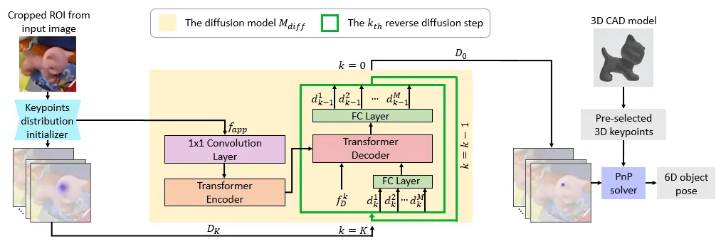
然而,直接从\(\hat{D}_K\)执行反向过程来生成\(D_0\)仍然可能存在困难,因为\(\hat{D}_K\)中缺少物体的外观特征。这些特征有助于基于输入图像来约束模型的反向过程,从而得到准确的预测结果。因此,我们进一步利用来自图像的外观特征作为上下文信息,以在反向过程中引导扩散模型\(M_\text{diff}\)。具体来说,我们重新利用从关键点分布初始化器中提取的特征作为外观特征\(f_\text{app}\),并将\(f_\text{app}\)输入到扩散模型中,如图3所示。
我们的反向过程旨在从不确定分布\(\hat{D}_K\)(训练期间)或\(D_K\)(测试期间)生成一个确定分布\(D_0\)。下面我们描述一下测试期间的反向过程。我们首先从输入图像中获取\(f_\text{app}\)。然后,为了帮助扩散模型学习在每个反向步骤中执行去噪操作,按照“Denoising Diffusion Probabilistic Models”的方法,我们生成唯一的步骤嵌入\(f_D^k\),以便将步骤编号(\(k\))信息注入到模型中。这样,给定从第\(k\)步的\(D_k\)中抽取的一组含噪关键点坐标\(d_k \in \mathbb{R}^{N \times 2}\),我们使用以步骤嵌入\(f_D^k\)和物体外观特征\(f_\text{app}\)为条件的扩散模型\(M_\text{diff}\),从\(d_k\)中恢复出\(d_{k - 1}\),如下所示:
\[ \begin{equation}\label{eq6} d_{k - 1} = M_\text{diff}(d_k, f_\text{app}, f_D^k) \end{equation} \]
3.3. Training and Testing
Training
按照“PVNet: Pixel-wise Voting Network for 6DoF Pose Estimation”的方法,我们首先使用最远点采样(FPS)算法从物体的CAD模型表面选取\(N\)个3D关键点。然后,我们分以下两个阶段进行训练过程。
在第一阶段,为了初始化分布\(D_K\),我们对关键点分布初始化器进行优化。
具体而言,对于每个训练样本,给定预先选择的\(N\)个3D关键点,我们可以利用真实的物体6D位姿来获取相应的\(N\)个2D关键点的真实坐标。
然后,对于每个关键点,基于其相应的真实坐标,我们按照“Making Deep Heatmaps Robust to Partial Occlusions for 3D Object Pose Estimation”的方法生成一个真实热图,用于训练初始化器。
因此,对于每个训练样本,我们生成\(N\)个真实热图(一个热图对应一个2D关键点)。通过这种方式,用于优化初始化器的损失函数\(L_\text{init}\)可以表示为:
\[ \begin{equation}\label{eq7} L_\text{init} = \Vert\mathbf{H}_\text{pred} - \mathbf{H}_\text{GT}\Vert_2^2 \end{equation} \]
其中,\(\mathbf{H}_\text{pred}\)和\(\mathbf{H}_\text{GT}\)分别表示预测的热图和真实的热图。
在第二阶段,我们对扩散模型\(M_\text{diff}\)进行优化。对于每个训练样本,为了优化\(M_\text{diff}\),我们执行以下步骤:
首先,将输入图像输入到一个现成的目标检测器中,然后把检测到的感兴趣区域(ROI)输入到已训练好的初始化器中,以获得\(N\)个热图。同时,我们也能得到外观特征\(f_\text{app}\)。
利用这\(N\)个预测的热图来初始化\(D_K\),并使用期望最大化(EM)类型的算法将\(D_K\)描述为柯西混合(MoC)分布\(\hat{D}_K\)。
基于\(\hat{D}_K\),我们使用真实关键点坐标\(d_0\),通过正向过程(公式\(\eqref{eq5}\),即\(\hat{d}_k = \sqrt{\bar{\alpha}_k}d_0 + (1 - \sqrt{\bar{\alpha}_k})\mu^{\text{MoC}} + \sqrt{1 - \bar{\alpha}_k}\epsilon^\text{MoC}\))直接生成\(M\)组\((\hat{d}_1, \cdots, \hat{d}_K)\)(即\(\{\hat{d}_1^i, \cdots, \hat{d}_K^i\}_{i = 1}^M\))。
接着,我们的目标是优化扩散模型\(M_\text{diff}\),以从\(\hat{d}_k^i\)迭代地恢复出\(\hat{d}_{k - 1}^i\)。遵循先前的扩散模型研究工作“Denoising Diffusion Probabilistic Models”,我们将用于优化\(M_\text{diff}\)的损失\(L_\text{diff}\)表述如下(对于所有的\(i\),\(\hat{d}_0^i = d_0\)):
\[ \begin{equation}\label{eq8} L_\text{diff} = \sum_{i = 1}^M \sum_{k = 1}^K \Vert M_\text{diff}(\hat{d}_k^i, f_\text{app}, f_D^k) - \hat{d}_{k - 1}^i\Vert_2^2 \end{equation} \]
Testing
在测试阶段,对于每个测试样本,将输入图像依次输入到目标检测器和关键点分布初始化器中,我们可以初始化分布\(D_K\),同时获取外观特征\(f_\text{app}\)。接着,我们执行反向过程。在反向过程中,我们从\(D_K\)中采样\(M\)组含噪的关键点坐标(即\(\{d_K^i\}_{i = 1}^M\)),并将它们输入到已训练好的扩散模型中。这里我们采样\(M\)组关键点坐标,是因为我们要从一个分布(\(D_K\))转换到另一个分布(\(D_0\))。然后,模型迭代地执行反向步骤。经过\(K\)步反向扩散后,我们得到\(M\)组预测的关键点坐标(即\(\{d_0^i\}_{i = 1}^M\))。为了得到最终的关键点坐标预测结果\(d_0\),我们计算这\(M\)个预测结果的均值。最后,我们可以像文献“PVNet: Pixel-wise Voting Network for 6DoF Pose Estimation”那样,使用PnP来计算物体的6D位姿。
3.4. Model Architecture
我们的框架主要由扩散模型(\(M_\text{diff}\))和关键点分布初始化器组成。
Diffusion Model \(M_\text{diff}\)
如图3所示,我们提出的扩散模型\(M_\text{diff}\)主要由一个Transformer编解码器架构组成。外观特征\(f_\text{app}\)被输入到编码器中,用于提取上下文信息,以辅助解码器进行反向过程。步骤嵌入\(f_D^k\)和\(\{d_k^i\}_{i = 1}^M\)(训练期间为\(\{\hat{d}_k^i\}_{i = 1}^M\))被输入到解码器中进行反向过程。编码器和解码器均包含由三个Transformer层组成的堆叠结构。
更具体地说,对于编码器部分,我们首先通过一个1×1卷积层将\(f_\text{app} \in \mathbb{R}^{16 \times 16 \times 512}\)映射为一个潜在嵌入\(e_\text{app} \in \mathbb{R}^{16 \times 16 \times 128}\)。为了保留空间信息,我们按照“Attention Is All You Need”的方法,进一步将位置编码融入到\(e_\text{app}\)中。之后,我们将\(e_\text{app}\)展平为一个特征序列(\(\mathbb{R}^{256 \times 128}\)),并将其输入到编码器中。包含所提取物体信息的编码器输出\(f_\text{enc}\)将被输入到解码器中,以辅助反向过程。需要注意的是,在测试期间,对于每个样本,我们仅需执行一次上述计算过程,即可获得相应的\(f_\text{enc}\)。
解码器部分会迭代地执行反向过程。为了简化表示,下面我们描述针对单个样本\(d_k\)而非\(M\)个样本(\(\{d_1^i, \cdots, d_K^i\}_{i = 1}^M\))的反向过程。具体而言,在第\(k\)个反向步骤中,为了将当前步骤编号(\(k\))的信息注入到解码器中,我们首先按照“Denoising Diffusion Probabilistic Models”的方法,使用正弦函数生成步骤嵌入\(f_D^k \in \mathbb{R}^{1 \times 128}\)。同时,我们使用一个全连接(FC)层将输入\(d_k \in \mathbb{R}^{N \times 2}\)映射为一个潜在嵌入\(e_k \in \mathbb{R}^{N \times 128}\)。然后,我们沿着第一个维度将\(f_D^k\)和\(e_k\)拼接起来,并将其输入到解码器中。通过在每一层利用交叉注意力机制与编码器输出\(f_\text{enc}\)(所提取的物体信息)进行交互,解码器会生成\(f_\text{dec}\),\(f_\text{dec}\)会进一步通过一个全连接层被映射为关键点坐标预测\(d_{k - 1} \in \mathbb{R}^{N \times 2}\)。接着,我们将\(d_{k - 1}\)作为输入反馈给解码器,以执行下一个反向步骤。
Keypoints Distribution Initializer
初始化器采用了ResNet-34骨干网络,这在6D位姿估计方法中是常用的(如文献“ZebraPose: Coarse to Fine Surface Encoding for 6DoF Object Pose Estimation”)。为了生成热图以初始化分布\(D_K\),我们在ResNet-34骨干网络之后添加了两个反卷积层,随后再接一个1×1卷积层,进而得到预测热图\(\mathbf{H}_\text{pred} \in \mathbb{R}^{N \times \frac{H}{4} \times \frac{W}{4}}\),其中\(H\)和\(W\)分别表示输入感兴趣区域(ROI)图像的高度和宽度。此外,ResNet-34骨干网络输出的特征,再结合通过文献“CheckerPose: Progressive Dense Keypoint Localization for Object Pose Estimation with Graph Neural Network”中的方法所获取的特征,被用作物体外观特征\(f_\text{app}\)。
4. Experiments
4.1. Datasets & Evaluation Metrics
4.2. Implementation Details
我们在英伟达V100 GPU上开展实验。我们将预先选定的三维关键点数量\(N\)设为128。在训练过程中,参照文献“CDPN: Coordinates-Based Disentangled Pose Network for Real-Time RGB-Based 6-DoF Object Pose Estimation”,我们采用动态缩放策略来生成增强的感兴趣区域(ROI)图像。在测试阶段,我们使用由CDPNv2提供的基于Faster RCNN和FCOS的检测框。裁剪后的ROI图像被调整为\(3 \times 256 \times 256\)的尺寸(\(H = W = 256\))。在正向扩散过程中,我们通过包含9个柯西核的柯西混合(MoC)模型(\(U = 9\))来描述\(D_K\)。我们使用Adam优化器对扩散模型\(M_\text{diff}\)进行1500个轮次的优化,初始学习率设为\(4 \times 10^{-5}\)。此外,我们将采样集的数量\(M\)设为5,扩散步数\(K\)设为100。参照文献“ZebraPose: Coarse to Fine Surface Encoding for 6DoF Object Pose Estimation”,我们使用Progressive-X作为PnP求解器。需要注意的是,在测试阶段,我们没有采用全部\(K\)步来执行反向过程,而是使用了最近提出的扩散加速方法DDIM来加速这一过程。借助DDIM加速,在测试时我们仅需执行10步就能完成反向过程。
4.3. Comparison with State-of-the-art Methods
| Method | PVNet [44] | HybridPose [51] | RePose [24] | DeepIM [33] | GDR-Net [61] | SO-Pose [8] | CRT-6D [4] | ZebraPose [53] | CheckerPose [35] | Ours |
|---|---|---|---|---|---|---|---|---|---|---|
| ape | 15.8 | 20.9 | 31.1 | 59.2 | 46.8 | 48.4 | 53.4 | 57.9 | 58.3 | 60.6 |
| can | 63.3 | 75.3 | 80.0 | 63.5 | 90.8 | 85.8 | 92.0 | 95.0 | 95.7 | 97.9 |
| cat | 16.7 | 24.9 | 25.6 | 26.2 | 40.5 | 32.7 | 42.0 | 60.6 | 62.3 | 63.2 |
| driller | 65.7 | 70.2 | 73.1 | 55.6 | 82.6 | 77.4 | 81.4 | 94.8 | 93.7 | 96.6 |
| duck | 25.2 | 27.9 | 43.0 | 52.4 | 46.9 | 48.9 | 44.9 | 64.5 | 69.9 | 67.2 |
| eggbox∗ | 50.2 | 52.4 | 51.7 | 63.0 | 54.2 | 52.4 | 62.7 | 70.9 | 70.0 | 73.5 |
| glue∗ | 49.6 | 53.8 | 54.3 | 71.7 | 75.8 | 78.3 | 80.2 | 88.7 | 86.4 | 92.0 |
| holepuncher | 39.7 | 54.2 | 53.6 | 52.5 | 60.1 | 75.3 | 74.3 | 83.0 | 83.8 | 85.5 |
| Mean | 40.8 | 47.5 | 51.6 | 55.5 | 62.2 | 62.3 | 66.3 | 76.9 | 77.5 | 79.6 |
| Method | ADD(-S) | AUC of ADD-S | AUC of ADD(-S) |
|---|---|---|---|
| SegDriven[21] | 39.0 | - | - |
| SingleStage[22] | 53.9 | - | - |
| CosyPose [29] | - | 89.8 | 84.5 |
| RePose [24] | 62.1 | 88.5 | 82.0 |
| GDR-Net [61] | 60.1 | 91.6 | 84.4 |
| SO-Pose [8] | 56.8 | 90.9 | 83.9 |
| ZebraPose [53] | 80.5 | 90.1 | 85.3 |
| CheckerPose [35] | 81.4 | 91.3 | 86.4 |
| Ours | 83.8 | 91.5 | 87.0 |
4.4. Ablation Studies
| Method | ADD(-S) |
|---|---|
| Variant A | 49.2 |
| Variant B | 57.3 |
| Variant C | 61.1 |
| 6D-Diff | 79.6 |
| Method | ADD(-S) |
|---|---|
| w/o \(f_\text{app}\) | 74.4 |
| 6D-Diff | 79.6 |
| Method | ADD(-S) |
|---|---|
| Standard diffusion w/o MoC | 73.1 |
| Heatmaps as condition | 76.2 |
| 6D-Diff | 79.6 |