【代码阅读】Instance-Adaptive and Geometric-Aware Keypoint Learning for Category-Level 6D Object Pose Estimation
数据处理
在./provider/create_dataloaders.py中创建Dataloader,分别可以使用camera_real,camera和housecat6d三种创建方式,如果使用camera_real方式创建的话,camera和real的比例为3:1。
深度图加载
由于该方法使用到了CAMERA25和REAL25两个数据集,而CAMERA25数据集是一个合成数据集,其深度图为合成深度图,所以需要进行处理,下面是合成深度图的读取方法(注意这里读取的是./data/camera_full_depths/中的图,和./data/camera/中的不一样):
1 | def load_composed_depth(img_path): |
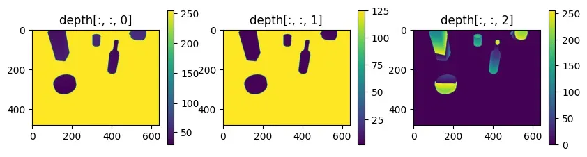
使用OpenCV读取./data/camera/train/00000/0000_depth.png,分别可视化其三个通道:
1 | import cv2 |
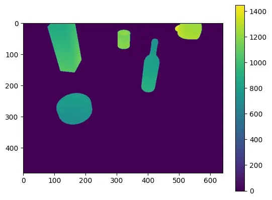
合成第1通道和第2通道:
1 | import cv2 |
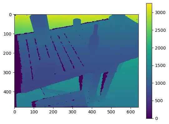
读取./data/camera_full_depths/train/00000/0000_composed.png,直接可视化:
1 | import cv2 |
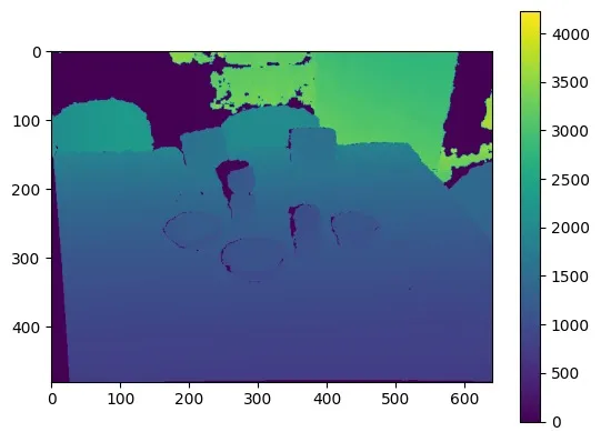
下面是真实深度图的读取方法:
1 | def load_depth(img_path): |
直接读取./data/real/train/scene_1/0000_depth.png并可视化:
1 | import cv2 |
简单来说就是合成数据集读取的是./data/camera_full_depths/中的深度图,而真实数据集读取的是./data/real/中的深度图。
深度图补全
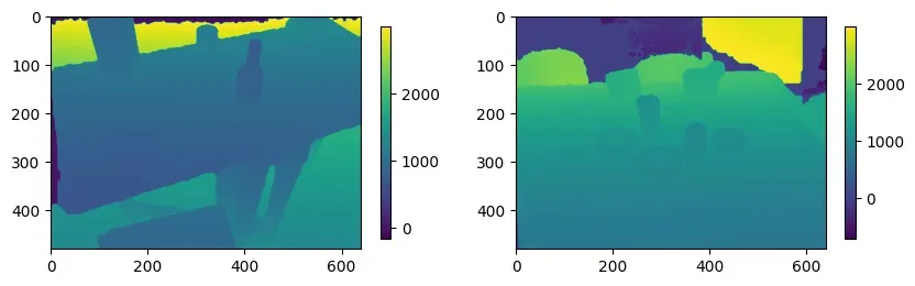
然后对深度图进行补全,分别对合成深度图和真实深度图进行补全:
1 | import matplotlib.pyplot as plt |
mask加载
以下读取./data/camera/train/00000/0000_label.pkl中的内容:
1 | with open(img_path + '_label.pkl', 'rb') as f: |
gts的内容为:
1 | {'class_ids': [1, 2, 6, 1], |
读取mask:
1 | mask = cv2.imread(img_path + '_mask.png')[:, :, 2] |
这里只取了第2通道,因为第2通道携带了类别信息:
1 | mask = cv2.imread('./data/camera/train/00000/0000_mask.png') |
与上方的instance_ids对应。
去除非目标物体的mask
首先随机选取一个物体(注意,训练时会从图像中所有物体中随机返回一个,而测试时则会全部返回):
1 | idx = np.random.randint(0, num_instance) |
使用get_bbox:
1 | rmin, rmax, cmin, cmax = get_bbox(gts['bboxes'][idx]) |
1 | def get_bbox(bbox): |
以原boundingbox的中心为中心,生成长宽为40的倍数的boundingbox,并考虑了结果boundingbox超出图像范围的情况。
使用与操作去除其余物体的mask:
1 | mask = np.equal(mask, gts['instance_ids'][idx]) |
从物体上采样
在后续得到物体点云后,需要从点云中采样固定数量的点以调整为网络需要的输入维度,在这一步实现。
1 | choose = mask[rmin:rmax, cmin:cmax].flatten().nonzero()[0] |
从mask中截取目标物体的一部分,然后展平,得到其非零值的下标。
采样到固定数量(配置文件中为1024):
1 | if len(choose) <= self.sample_num: # 1024 |
将深度图转换为点云
获取内参:
1 | cam_fx, cam_fy, cam_cx, cam_cy = self.intrinsics |
(深度)归一化:
1 | pts2 = depth.copy() / self.norm_scale |
将像素坐标系中的xy坐标转换为相机坐标系中的xy坐标:
1 | self.xmap = np.array([[i for i in range(640)] for j in range(480)]) |
具体原理见:针孔相机成像模型
合并并裁剪:
1 | pts = np.transpose(np.stack([pts0, pts1, pts2]), (1, 2, 0)).astype(np.float32) |
RGB
这里会将目标图像使用rmin, rmax, cmin, cmax进行裁剪,然后resize(代码中为\(224 \times
224\)),那么相应的采样下标也需要修改。
除此之外,使用OpenCV读入RGB时,其维度顺序为HWC,在经过transforms.ToTensor()后,维度顺序会变为CHW。
修改采样下标
1 | crop_w = rmax - rmin # 原本crop mask的宽度 |
读取物体模型点云
首先是全部物体的模型点云,这里读取的是./data/obj_models/camera_train.pkl中的数据:
1 | self.models = {} |
该文件以字典的形式存储了物体的点云信息,可以通过键取出对应的点云:
1 | model = self.models[gts['model_list'][idx]].astype(np.float32) |
取出物体的平移、旋转和大小:
1 | translation = gts['translations'][idx].astype(np.float32) # 3 物体坐标系到相机坐标系的平移 |
处理对称物体
1 | if cat_id in self.sym_ids: |
Y轴朝上,所以第2列为\([0, 1, 0]\)。
网络架构
RGB特征
使用DINOv2提取RGB特征:
1 | self.rgb_extractor = torch.hub.load('facebookresearch/dinov2','dinov2_vits14') |
还使用了一个1d卷积:
1 | self.feature_mlp = nn.Sequential( |
挑选RGB特征
在数据处理时,生成了一个choose变量,这里要用该变量将RGB特征从\(\mathbb{R}^{b \times 128 \times (196 \times
196)}\)采样为\(\mathbb{R}^{b \times 128
\times 1024}\)。
加噪
1 | if self.training: |
其中,生成噪声的函数为:
1 | def generate_augmentation(batchsize): |
模型会预测加噪后的位姿,然后在Loss阶段,会使用生成的噪声去除噪声,以实现数据增强。
点云特征
原文中说使用PointNet++来提取点云特征,但是暂时没有阅读过和PointNet++相关的论文,所以暂时不详细写。
IAKD
该模块以RGB特征和点云特征为输入,将点云特征和RGB特征进行拼接后作为\(KV\)、将可训练的一个查询向量作为\(Q\),执行交叉注意力,返回处理后的查询向量和注意力图。
然后使用查询向量和输入特征做矩阵乘法,得到热图,最后返回查询向量和热图。
热图将拼接后的点云特征和RGB特征进一步压缩。
GAFA
首先使用一堆卷积和一堆全连接堆叠成GAFA块,然后使用两个GAFA块组成GAFA模块,最后返回关键点特征。
训练
这里训练和测试都使用的是Gorilla-Lab-SCUT/gorilla-core中的包。